PCA (Principal Component Analysis)#
Links: notebook, html, PDF, python, slides, GitHub
This notebook shows how to plot a PCA with sciki-learn and statsmodels, with or without normalization.
%matplotlib inline
import matplotlib.pyplot as plt
plt.style.use('ggplot')
from jyquickhelper import add_notebook_menu
add_notebook_menu()
More about PCA: Implementing a Principal Component Analysis (PCA) in Python step by step.
Download data#
import pyensae.datasource
pyensae.datasource.download_data("auto-mpg.data", url="https://archive.ics.uci.edu/ml/machine-learning-databases/auto-mpg/")
'auto-mpg.data'
import pandas
df = pandas.read_fwf("auto-mpg.data", encoding="utf-8",
                    names="mpg cylinders displacement horsepower weight acceleration year origin name".split())
df["name"] = df["name"].apply(lambda s : s.strip(' "'))
df.head()
| mpg | cylinders | displacement | horsepower | weight | acceleration | year | origin | name | |
|---|---|---|---|---|---|---|---|---|---|
| 0 | 18.0 | 8 | 307.0 | 130.0 | 3504.0 | 12.0 | 70 | 1 | chevrolet chevelle malibu |
| 1 | 15.0 | 8 | 350.0 | 165.0 | 3693.0 | 11.5 | 70 | 1 | buick skylark 320 |
| 2 | 18.0 | 8 | 318.0 | 150.0 | 3436.0 | 11.0 | 70 | 1 | plymouth satellite |
| 3 | 16.0 | 8 | 304.0 | 150.0 | 3433.0 | 12.0 | 70 | 1 | amc rebel sst |
| 4 | 17.0 | 8 | 302.0 | 140.0 | 3449.0 | 10.5 | 70 | 1 | ford torino |
df.dtypes
mpg             float64
cylinders         int64
displacement    float64
horsepower       object
weight          float64
acceleration    float64
year              int64
origin            int64
name             object
dtype: object
We remove missing values:
df[df.horsepower == "?"]
| mpg | cylinders | displacement | horsepower | weight | acceleration | year | origin | name | |
|---|---|---|---|---|---|---|---|---|---|
| 32 | 25.0 | 4 | 98.0 | ? | 2046.0 | 19.0 | 71 | 1 | ford pinto |
| 126 | 21.0 | 6 | 200.0 | ? | 2875.0 | 17.0 | 74 | 1 | ford maverick |
| 330 | 40.9 | 4 | 85.0 | ? | 1835.0 | 17.3 | 80 | 2 | renault lecar deluxe |
| 336 | 23.6 | 4 | 140.0 | ? | 2905.0 | 14.3 | 80 | 1 | ford mustang cobra |
| 354 | 34.5 | 4 | 100.0 | ? | 2320.0 | 15.8 | 81 | 2 | renault 18i |
| 374 | 23.0 | 4 | 151.0 | ? | 3035.0 | 20.5 | 82 | 1 | amc concord dl |
final = df[df.horsepower != '?'].copy()
final["horsepower"] = final["horsepower"].astype(float)
final.to_csv("auto-mpg.data.csv", sep="\t", index=False, encoding="utf-8")
final.shape
(392, 9)
PCA with scikit-learn#
from sklearn.decomposition import PCA
X = final[df.columns[1:-1]]
Y = final["mpg"]
pca = PCA(n_components=2)
pca.fit(X)
PCA(copy=True, iterated_power='auto', n_components=2, random_state=None,
  svd_solver='auto', tol=0.0, whiten=False)
out = pca.transform(X)
out[:5]
array([[536.44492922,  50.83312832],
       [730.34140206,  79.13543921],
       [470.9815846 ,  75.4476722 ],
       [466.40143367,  62.53420646],
       [481.66788465,  55.78036021]])
pca.explained_variance_ratio_, pca.noise_variance_
(array([0.99756151, 0.0020628 ]), 55.14787750463889)
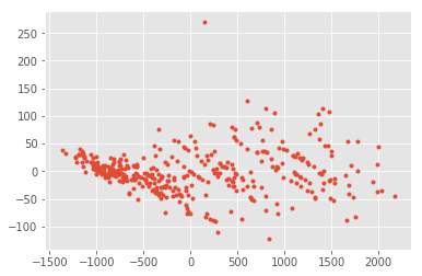
import matplotlib.pyplot as plt
plt.plot(out[:,0], out[:,1], ".");
pca.components_
array([[ 1.79262233e-03,  1.14341275e-01,  3.89670355e-02,
         9.92673415e-01, -1.35283460e-03, -1.33684138e-03,
        -5.51538021e-04],
       [ 1.33244815e-02,  9.45778439e-01,  2.98248416e-01,
        -1.20752748e-01, -3.48258394e-02, -2.38516836e-02,
        -3.24298106e-03]])
PCA with scikit-learn and normalization#
from sklearn.decomposition import PCA
from sklearn.preprocessing import Normalizer
from sklearn.pipeline import Pipeline

normpca = Pipeline([('norm', Normalizer()), ('pca', PCA(n_components=2))])
normpca.fit(X)
Pipeline(memory=None,
     steps=[('norm', Normalizer(copy=True, norm='l2')), ('pca', PCA(copy=True, iterated_power='auto', n_components=2, random_state=None,
  svd_solver='auto', tol=0.0, whiten=False))])
out = normpca.transform(X)
out[:5]
array([[0.02731781, 0.00012872],
       [0.03511968, 0.00666259],
       [0.03247168, 0.00632048],
       [0.0287677 , 0.0060517 ],
       [0.02758449, 0.00325874]])
normpca.named_steps['pca'].explained_variance_ratio_, normpca.named_steps['pca'].noise_variance_
(array([0.86819249, 0.08034075]), 4.332607718595102e-06)
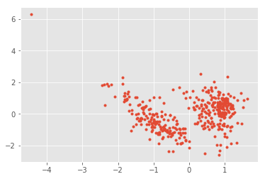
import matplotlib.pyplot as plt
plt.plot(out[:,0], out[:,1], ".");
normpca.named_steps['pca'].components_
array([[ 0.00415209,  0.92648229,  0.11272098, -0.05732771, -0.09162071,
        -0.34198745, -0.01646403],
       [ 0.01671457,  0.0789351 ,  0.85881718, -0.06957932,  0.02998247,
         0.49941847,  0.02763848]])
PCA with statsmodels#
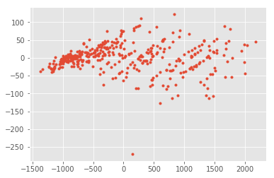
from statsmodels.sandbox.tools import pca
xred, fact, eva, eve = pca(X, keepdim=2, normalize=False)
fact[:5]
array([[536.44492922, -50.83312832],
       [730.34140206, -79.13543921],
       [470.9815846 , -75.4476722 ],
       [466.40143367, -62.53420646],
       [481.66788465, -55.78036021]])
eva
array([732151.6743476 , 1513.97202164])
eve
array([[ 1.79262233e-03, -1.33244815e-02],
       [ 1.14341275e-01, -9.45778439e-01],
       [ 3.89670355e-02, -2.98248416e-01],
       [ 9.92673415e-01,  1.20752748e-01],
       [-1.35283460e-03,  3.48258394e-02],
       [-1.33684138e-03,  2.38516836e-02],
       [-5.51538021e-04,  3.24298106e-03]])
plt.plot(fact[:,0], fact[:,1], ".");
PCA with statsmodels and normalization#
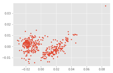
from statsmodels.sandbox.tools import pca
from sklearn.preprocessing import normalize
X_norm = normalize(X)
xred, fact, eva, eve = pca(X_norm, keepdim=2, normalize=True)
eva
array([3.65433661e-04, 3.38164814e-05])
eve
array([[ -0.21720145,   2.87429329],
       [-48.46551687,  13.57394009],
       [ -5.89658384, 147.68504393],
       [  2.99888854, -11.96508998],
       [  4.79280102,   5.15588534],
       [ 17.88981698,  85.8816515 ],
       [  0.86125514,   4.75280519]])
plt.plot(fact[:,0], fact[:,1], ".");