2A.ML101.5: Measuring prediction performance#

Links: notebook, html, python, slides, GitHub

Source: Course on machine learning with scikit-learn by Gaël Varoquaux

Using the K-neighbors classifier#

Here we’ll continue to look at the digits data, but we’ll switch to the K-Neighbors classifier. The K-neighbors classifier is an instance-based classifier. The K-neighbors classifier predicts the label of an unknown point based on the labels of the K nearest points in the parameter space.

# Get the data
from sklearn.datasets import load_digits
digits = load_digits()
X = digits.data
y = digits.target

# Instantiate and train the classifier
from sklearn.neighbors import KNeighborsClassifier
clf = KNeighborsClassifier(n_neighbors=1)
clf.fit(X, y)

KNeighborsClassifier(n_neighbors=1)

In a Jupyter environment, please rerun this cell to show the HTML representation or trust the notebook.
On GitHub, the HTML representation is unable to render, please try loading this page with nbviewer.org.

# Check the results using metrics
from sklearn import metrics
y_pred = clf.predict(X)

print(metrics.confusion_matrix(y_pred, y))

[[178   0   0   0   0   0   0   0   0   0]
 [  0 182   0   0   0   0   0   0   0   0]
 [  0   0 177   0   0   0   0   0   0   0]
 [  0   0   0 183   0   0   0   0   0   0]
 [  0   0   0   0 181   0   0   0   0   0]
 [  0   0   0   0   0 182   0   0   0   0]
 [  0   0   0   0   0   0 181   0   0   0]
 [  0   0   0   0   0   0   0 179   0   0]
 [  0   0   0   0   0   0   0   0 174   0]
 [  0   0   0   0   0   0   0   0   0 180]]

Apparently, we’ve found a perfect classifier! But this is misleading for the reasons we saw before: the classifier essentially “memorizes” all the samples it has already seen. To really test how well this algorithm does, we need to try some samples it hasn’t yet seen.

This problem can also occur with regression models. In the following we fit an other instance-based model named “decision tree” to the Diabete dataset we introduced previously:

%matplotlib inline
from matplotlib import pyplot as plt
import numpy as np

from sklearn.datasets import load_diabetes
from sklearn.tree import DecisionTreeRegressor

data = load_diabetes()
clf = DecisionTreeRegressor().fit(data.data, data.target)
predicted = clf.predict(data.data)
expected = data.target

plt.scatter(expected, predicted)
plt.plot([0, 350], [0, 350], '--k')
plt.axis('tight')
plt.xlabel('True Progression')
plt.ylabel('Predicted Progression');

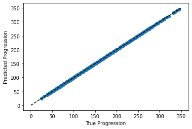
../_images/05_measuring_prediction_performance_10_0.png

Here again the predictions are seemingly perfect as the model was able to perfectly memorize the training set.

A Better Approach: Using a validation set#

Learning the parameters of a prediction function and testing it on the same data is a methodological mistake: a model that would just repeat the labels of the samples that it has just seen would have a perfect score but would fail to predict anything useful on yet-unseen data.

To avoid over-fitting, we have to define two different sets:

a training set X_train, y_train which is used for learning the parameters of a predictive model
a testing set X_test, y_test which is used for evaluating the fitted predictive model

In scikit-learn such a random split can be quickly computed with the train_test_split helper function. It can be used this way:

from sklearn.model_selection import train_test_split
X = digits.data
y = digits.target

X_train, X_test, y_train, y_test = train_test_split(X, y, test_size=0.25, random_state=0)

print("%r, %r, %r" % (X.shape, X_train.shape, X_test.shape))

(1797, 64), (1347, 64), (450, 64)

Now we train on the training data, and test on the testing data:

clf = KNeighborsClassifier(n_neighbors=1).fit(X_train, y_train)
y_pred = clf.predict(X_test)

print(metrics.confusion_matrix(y_test, y_pred))

[[37  0  0  0  0  0  0  0  0  0]
 [ 0 43  0  0  0  0  0  0  0  0]
 [ 0  0 43  1  0  0  0  0  0  0]
 [ 0  0  0 45  0  0  0  0  0  0]
 [ 0  0  0  0 38  0  0  0  0  0]
 [ 0  0  0  0  0 47  0  0  0  1]
 [ 0  0  0  0  0  0 52  0  0  0]
 [ 0  0  0  0  0  0  0 48  0  0]
 [ 0  0  0  0  0  0  0  0 48  0]
 [ 0  0  0  1  0  1  0  0  0 45]]

print(metrics.classification_report(y_test, y_pred))

              precision    recall  f1-score   support
           0       1.00      1.00      1.00        37
           1       1.00      1.00      1.00        43
           2       1.00      0.98      0.99        44
           3       0.96      1.00      0.98        45
           4       1.00      1.00      1.00        38
           5       0.98      0.98      0.98        48
           6       1.00      1.00      1.00        52
           7       1.00      1.00      1.00        48
           8       1.00      1.00      1.00        48
           9       0.98      0.96      0.97        47
    accuracy                           0.99       450
   macro avg       0.99      0.99      0.99       450
weighted avg       0.99      0.99      0.99       450

The averaged f1-score is often used as a convenient measure of the overall performance of an algorithm. It appears in the bottom row of the classification report; it can also be accessed directly:

metrics.f1_score(y_test, y_pred, average="macro")

0.9913675218842191

The over-fitting we saw previously can be quantified by computing the f1-score on the training data itself:

metrics.f1_score(y_train, clf.predict(X_train), average="macro")

1.0

Regression metrics In the case of regression models, we need to use different metrics, such as explained variance.

Application: Model Selection via Validation#

In the previous notebook, we saw Gaussian Naive Bayes classification of the digits. Here we saw K-neighbors classification of the digits. We’ve also seen support vector machine classification of digits. Now that we have these validation tools in place, we can ask quantitatively which of the three estimators works best for the digits dataset.

With the default hyper-parameters for each estimator, which gives the best f1 score on the validation set? Recall that hyperparameters are the parameters set when you instantiate the classifier: for example, the n_neighbors in
```
clf = KNeighborsClassifier(n_neighbors=1)
```
For each classifier, which value for the hyperparameters gives the best results for the digits data? For LinearSVC, use loss='l2' and loss='l1'. For KNeighborsClassifier we use n_neighbors between 1 and 10. Note that GaussianNB does not have any adjustable hyperparameters.

from sklearn.svm import LinearSVC
from sklearn.naive_bayes import GaussianNB
from sklearn.neighbors import KNeighborsClassifier

import warnings  # suppress warnings from older versions of KNeighbors
warnings.filterwarnings('ignore', message='kneighbors*')

X = digits.data
y = digits.target
X_train, X_test, y_train, y_test = train_test_split(X, y, test_size=0.25, random_state=0)

for Model in [LinearSVC, GaussianNB, KNeighborsClassifier]:
    clf = Model().fit(X_train, y_train)
    y_pred = clf.predict(X_test)
    print(Model.__name__,
          metrics.f1_score(y_test, y_pred, average="macro"))

print('------------------')

# test SVC loss
for loss, p, dual in [('squared_hinge', 'l1', False), ('squared_hinge', 'l2', True)]:
    clf = LinearSVC(penalty=p, loss=loss, dual=dual)
    clf.fit(X_train, y_train)
    y_pred = clf.predict(X_test)
    print("LinearSVC(penalty='{0}', loss='{1}')".format(p, loss),
          metrics.f1_score(y_test, y_pred, average="macro"))

print('-------------------')

# test K-neighbors
for n_neighbors in range(1, 11):
    clf = KNeighborsClassifier(n_neighbors=n_neighbors).fit(X_train, y_train)
    y_pred = clf.predict(X_test)
    print("KNeighbors(n_neighbors={0})".format(n_neighbors),
          metrics.f1_score(y_test, y_pred, average="macro"))

C:xavierdupre__home_github_forkscikit-learnsklearnsvm_base.py:1244: ConvergenceWarning: Liblinear failed to converge, increase the number of iterations.
  warnings.warn(

LinearSVC 0.9257041879239652
GaussianNB 0.8332741681010101
KNeighborsClassifier 0.9804562804949924
------------------

C:xavierdupre__home_github_forkscikit-learnsklearnsvm_base.py:1244: ConvergenceWarning: Liblinear failed to converge, increase the number of iterations.
  warnings.warn(
C:xavierdupre__home_github_forkscikit-learnsklearnsvm_base.py:1244: ConvergenceWarning: Liblinear failed to converge, increase the number of iterations.
  warnings.warn(

LinearSVC(penalty='l1', loss='squared_hinge') 0.9447242283258508
LinearSVC(penalty='l2', loss='squared_hinge') 0.9385749925598466
-------------------
KNeighbors(n_neighbors=1) 0.9913675218842191
KNeighbors(n_neighbors=2) 0.9848442068835102
KNeighbors(n_neighbors=3) 0.9867753449543099
KNeighbors(n_neighbors=4) 0.9803719053818863
KNeighbors(n_neighbors=5) 0.9804562804949924
KNeighbors(n_neighbors=6) 0.9757924194139573
KNeighbors(n_neighbors=7) 0.9780645792142071
KNeighbors(n_neighbors=8) 0.9780645792142071
KNeighbors(n_neighbors=9) 0.9780645792142071
KNeighbors(n_neighbors=10) 0.9755550897728812

Cross-validation#

Cross-validation consists in repetively splitting the data in pairs of train and test sets, called ‘folds’. Scikit-learn comes with a function to automatically compute score on all these folds. Here we do ‘K-fold’ with k=5.

clf = KNeighborsClassifier()
from sklearn.model_selection import cross_val_score
cross_val_score(clf, X, y, cv=5)

array([0.94722222, 0.95555556, 0.96657382, 0.98050139, 0.9637883 ])

We can use different splitting strategies, such as random splitting

from sklearn.model_selection import ShuffleSplit
cv = ShuffleSplit(n_splits=5)
cross_val_score(clf, X, y, cv=cv)

array([0.98333333, 0.98333333, 0.98888889, 0.98333333, 1.        ])

There exists many different cross-validation strategies in scikit-learn. They are often useful to take in account non iid datasets.

Hyperparameter optimization with cross-validation#

Consider regularized linear models, such as Ridge Regression, which uses $\ell_2$ regularlization, and Lasso Regression, which uses $\ell_1$ regularization. Choosing their regularization parameter is important.

Let us set these paramaters on the Diabetes dataset, a simple regression problem. The diabetes data consists of 10 physiological variables (age, sex, weight, blood pressure) measure on 442 patients, and an indication of disease progression after one year:

from sklearn.datasets import load_diabetes
data = load_diabetes()
X, y = data.data, data.target
print(X.shape)

(442, 10)

With the default hyper-parameters: we use the cross-validation score to determine goodness-of-fit:

from sklearn.linear_model import Ridge, Lasso

for Model in [Ridge, Lasso]:
    model = Model()
    print(Model.__name__, cross_val_score(model, X, y).mean())

Ridge 0.410174971340889
Lasso 0.3375593674654274

Basic Hyperparameter Optimization#

We compute the cross-validation score as a function of alpha, the strength of the regularization for Lasso and Ridge. We choose 20 values of alpha between 0.0001 and 1:

alphas = np.logspace(-3, -1, 30)

for Model in [Lasso, Ridge]:
    scores = [cross_val_score(Model(alpha), X, y, cv=3).mean()
              for alpha in alphas]
    plt.plot(alphas, scores, label=Model.__name__)
plt.legend(loc='lower left');

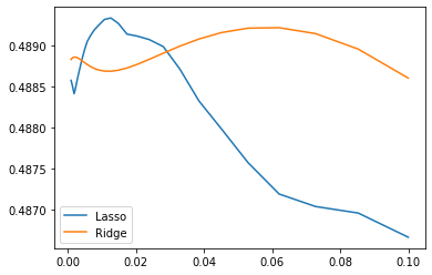
../_images/05_measuring_prediction_performance_40_0.png

Can we trust our results to be actually useful?

Automatically Performing Grid Search#

from sklearn.model_selection import GridSearchCV

GridSearchCV is constructed with an estimator, as well as a dictionary of parameter values to be searched. We can find the optimal parameters this way:

for Model in [Ridge, Lasso]:
    gscv = GridSearchCV(Model(), dict(alpha=alphas), cv=3).fit(X, y)
    print(Model.__name__, gscv.best_params_)

Ridge {'alpha': 0.06210169418915616}
Lasso {'alpha': 0.01268961003167922}

Built-in Hyperparameter Search#

For some models within scikit-learn, cross-validation can be performed more efficiently on large datasets. In this case, a cross-validated version of the particular model is included. The cross-validated versions of Ridge and Lasso are RidgeCV and LassoCV, respectively. The grid search on these estimators can be performed as follows:

from sklearn.linear_model import RidgeCV, LassoCV
for Model in [RidgeCV, LassoCV]:
    model = Model(alphas=alphas, cv=3).fit(X, y)
    print(Model.__name__, model.alpha_)

RidgeCV 0.06210169418915616
LassoCV 0.01268961003167922

We see that the results match those returned by GridSearchCV

Nested cross-validation#

How do we measure the performance of these estimators? We have used data to set the hyperparameters, so we need to test on actually new data. We can do this by running cross_val_score on our CV objects. Here there are 2 cross-validation loops going on, this is called ‘nested cross validation’:

for Model in [RidgeCV, LassoCV]:
    scores = cross_val_score(Model(alphas=alphas, cv=3), X, y, cv=3)
    print(Model.__name__, np.mean(scores))

RidgeCV 0.48916033973224776
LassoCV 0.4854908670556423

Note that these results do not match the best results of our curves above, and LassoCV seems to under-perform RidgeCV. The reason is that setting the hyper-parameter is harder for Lasso, thus the estimation error on this hyper-parameter is larger.

Liens

Contenu

Information

Sujet précédent

Sujet suivant