Pivot de gauss avec numpy#
Links: notebook, html, python, slides, GitHub
Etape par étape, le pivote de Gauss implémenté en python puis avec numpy.
from jyquickhelper import add_notebook_menu
add_notebook_menu()
%matplotlib inline
Python#
import numpy
def pivot_gauss(m):
    n = m.copy()
    for i in range(1, m.shape[0]):
        j0 = i
        while j0 < m.shape[0] and m[j0, i-1] == 0:
            j0 += 1
        for j in range(j0, m.shape[0]):
            coef = - m[j, i-1] / m[i-1, i-1]
            for k in range(i-1, m.shape[1]):
                m[j, k] += coef * m[i-1, k]
    return m


m = numpy.random.rand(4, 4)
piv = pivot_gauss(m)
piv * (numpy.abs(piv) > 1e-10)
array([[0.55773852, 0.26401337, 0.36548134, 0.12568338],
       [0.        , 0.84501794, 0.3183026 , 0.11992052],
       [0.        , 0.        , 0.26876495, 0.1272863 ],
       [0.        , 0.        , 0.        , 0.3082964 ]])
* (numpy.abs(piv) > 1e-10) sert à simplifier l’affichage des valeurs
quasi nulles.
Numpy 1#
def pivot_gauss2(m):
    n = m.copy()
    for i in range(1, m.shape[0]):
        j0 = i
        while j0 < m.shape[0] and m[j0, i-1] == 0:
            j0 += 1
        for j in range(j0, m.shape[0]):
            coef = - m[j, i-1] / m[i-1, i-1]
            m[j, i-1:] += m[i-1, i-1:] * coef
    return m


piv = pivot_gauss2(m)
piv * (numpy.abs(piv) > 1e-10)
array([[0.55773852, 0.26401337, 0.36548134, 0.12568338],
       [0.        , 0.84501794, 0.3183026 , 0.11992052],
       [0.        , 0.        , 0.26876495, 0.1272863 ],
       [0.        , 0.        , 0.        , 0.3082964 ]])
Numpy 2#
def pivot_gauss3(m):
    n = m.copy()
    for i in range(1, m.shape[0]):
        j0 = i
        while j0 < m.shape[0] and m[j0, i-1] == 0:
            j0 += 1
        coef = - m[j0:, i-1] / m[i-1, i-1]
        m[j0:, i-1:] += coef.reshape((-1, 1)) * m[i-1, i-1:].reshape((1, -1))
    return m


piv = pivot_gauss3(m)
piv * (numpy.abs(piv) > 1e-10)
array([[0.55773852, 0.26401337, 0.36548134, 0.12568338],
       [0.        , 0.84501794, 0.3183026 , 0.11992052],
       [0.        , 0.        , 0.26876495, 0.1272863 ],
       [0.        , 0.        , 0.        , 0.3082964 ]])
Vitesse#
from cpyquickhelper.numbers import measure_time
from tqdm import tqdm
import pandas

data = []
for n in tqdm([10, 20, 30, 40, 50, 60, 70, 80, 100]):
    m = numpy.random.rand(n, n)
    if n < 50:
        res = measure_time(lambda: pivot_gauss(m), number=10, repeat=10)
        res.update(dict(name="python", n=n))
        data.append(res)
    res = measure_time(lambda: pivot_gauss2(m), number=10, repeat=10)
    res.update(dict(name="numpy1", n=n))
    data.append(res)
    res = measure_time(lambda: pivot_gauss3(m), number=10, repeat=10)
    res.update(dict(name="numpy2", n=n))
    data.append(res)

df = pandas.DataFrame(data)
df
100%|██████████| 9/9 [00:04<00:00, 1.82it/s]
| average | deviation | min_exec | max_exec | repeat | number | ttime | context_size | name | n | |
|---|---|---|---|---|---|---|---|---|---|---|
| 0 | 0.000674 | 0.000213 | 0.000374 | 0.001088 | 10 | 10 | 0.006741 | 64 | python | 10 |
| 1 | 0.000454 | 0.000127 | 0.000256 | 0.000562 | 10 | 10 | 0.004544 | 64 | numpy1 | 10 |
| 2 | 0.001363 | 0.000390 | 0.000780 | 0.001894 | 10 | 10 | 0.013629 | 64 | numpy2 | 10 |
| 3 | 0.001038 | 0.000959 | 0.000658 | 0.003908 | 10 | 10 | 0.010384 | 64 | python | 20 |
| 4 | 0.000841 | 0.000280 | 0.000656 | 0.001640 | 10 | 10 | 0.008413 | 64 | numpy1 | 20 |
| 5 | 0.001814 | 0.000280 | 0.001621 | 0.002472 | 10 | 10 | 0.018138 | 64 | numpy2 | 20 |
| 6 | 0.013065 | 0.009250 | 0.007522 | 0.033579 | 10 | 10 | 0.130650 | 64 | python | 30 |
| 7 | 0.003207 | 0.000164 | 0.002992 | 0.003397 | 10 | 10 | 0.032071 | 64 | numpy1 | 30 |
| 8 | 0.002815 | 0.000030 | 0.002782 | 0.002874 | 10 | 10 | 0.028153 | 64 | numpy2 | 30 |
| 9 | 0.053362 | 0.020418 | 0.040569 | 0.099695 | 10 | 10 | 0.533620 | 64 | python | 40 |
| 10 | 0.012710 | 0.001281 | 0.011835 | 0.015254 | 10 | 10 | 0.127104 | 64 | numpy1 | 40 |
| 11 | 0.005585 | 0.000941 | 0.004866 | 0.007821 | 10 | 10 | 0.055855 | 64 | numpy2 | 40 |
| 12 | 0.024682 | 0.005618 | 0.019726 | 0.036658 | 10 | 10 | 0.246824 | 64 | numpy1 | 50 |
| 13 | 0.007721 | 0.000831 | 0.007127 | 0.010041 | 10 | 10 | 0.077207 | 64 | numpy2 | 50 |
| 14 | 0.038531 | 0.006086 | 0.032592 | 0.053980 | 10 | 10 | 0.385306 | 64 | numpy1 | 60 |
| 15 | 0.009483 | 0.000068 | 0.009380 | 0.009618 | 10 | 10 | 0.094831 | 64 | numpy2 | 60 |
| 16 | 0.042429 | 0.008567 | 0.035483 | 0.063337 | 10 | 10 | 0.424291 | 64 | numpy1 | 70 |
| 17 | 0.011983 | 0.000712 | 0.011418 | 0.013913 | 10 | 10 | 0.119831 | 64 | numpy2 | 70 |
| 18 | 0.084926 | 0.009155 | 0.076947 | 0.106115 | 10 | 10 | 0.849257 | 64 | numpy1 | 80 |
| 19 | 0.015445 | 0.000432 | 0.014988 | 0.016419 | 10 | 10 | 0.154452 | 64 | numpy2 | 80 |
| 20 | 0.137455 | 0.007508 | 0.122579 | 0.148460 | 10 | 10 | 1.374552 | 64 | numpy1 | 100 |
| 21 | 0.025048 | 0.000231 | 0.024841 | 0.025697 | 10 | 10 | 0.250484 | 64 | numpy2 | 100 |
piv = df.pivot(index="n", columns="name", values="average")
piv
| name | numpy1 | numpy2 | python |
|---|---|---|---|
| n | |||
| 10 | 0.000454 | 0.001363 | 0.000674 |
| 20 | 0.000841 | 0.001814 | 0.001038 |
| 30 | 0.003207 | 0.002815 | 0.013065 |
| 40 | 0.012710 | 0.005585 | 0.053362 |
| 50 | 0.024682 | 0.007721 | NaN |
| 60 | 0.038531 | 0.009483 | NaN |
| 70 | 0.042429 | 0.011983 | NaN |
| 80 | 0.084926 | 0.015445 | NaN |
| 100 | 0.137455 | 0.025048 | NaN |
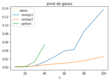
piv.plot(title="pivot de gauss");