2016 - Une solution à la compétition de machine learning 2A#

Links: notebook, html, python, slides, GitHub

Ce notebook a été proposé par un étudiant pour la compétition organisée pour ce cours : classification binaire.

from pyensae.datasource import download_data
download_data("ensae_competition_2016.zip",
              url="https://github.com/sdpython/ensae_teaching_cs/raw/master/_doc/competitions/2016_ENSAE_2A/")

['ensae_competition_test_X.txt', 'ensae_competition_train.txt']

# packages
import pandas as pd
import numpy as np
from sklearn import svm, linear_model, datasets, metrics
import seaborn as sns
import matplotlib.pyplot as plt
%matplotlib inline
from statsmodels.nonparametric.kde import KDEUnivariate
from statsmodels.nonparametric import smoothers_lowess

# dataframe
# df = pd.read_excel("default_of_credit_card_clients.xls", header=[0, 1], encoding="utf8", index_col=0, engine='openpyxl')
df = pd.read_csv("ensae_competition_train.txt", header=[0, 1], encoding="utf8", index_col=0, sep="\t")
df.head(10)

	X1	X2	X3	X4	X5	X6	X7	X8	X9	X10	...	X15	X16	X17	X18	X19	X20	X21	X22	X23	Y
ID	LIMIT_BAL	SEX	EDUCATION	MARRIAGE	AGE	PAY_0	PAY_2	PAY_3	PAY_4	PAY_5	...	BILL_AMT4	BILL_AMT5	BILL_AMT6	PAY_AMT1	PAY_AMT2	PAY_AMT3	PAY_AMT4	PAY_AMT5	PAY_AMT6	default payment next month
0	180000	1	2	1	47	0	0	0	0	0	...	99694	65977	67415	3700	3700	4100	2360	2500	2618	0
1	110000	2	2	1	35	0	0	0	0	0	...	4869	4966	5070	1053	1073	1081	178	184	185	1
2	70000	2	2	2	22	0	0	0	0	0	...	69927	50579	49483	2501	3001	2608	1777	1792	1793	1
3	200000	2	1	2	27	-2	-2	-2	-2	-2	...	1665	3370	-36	5610	15616	1673	3385	0	95456	0
4	370000	2	1	1	39	0	0	0	0	0	...	48216	47675	48074	2157	2000	1668	2000	3000	1000	0
5	260000	2	1	1	29	0	0	0	-2	-2	...	0	0	0	3090	0	0	0	0	141516	0
6	90000	2	1	1	43	-1	-1	2	-1	-1	...	7660	21175	4009	4367	9	7660	21175	4009	7452	0
7	220000	2	1	1	43	-1	3	2	0	0	...	1090	1090	0	167	0	0	0	0	0	1
8	50000	1	2	1	35	1	2	0	0	0	...	21260	70	29575	0	2052	1800	0	29935	1200	1
9	50000	2	3	2	40	0	0	0	0	0	...	8292	8465	8650	1271	1130	1000	307	325	436	0

10 rows × 24 columns

df.columns

MultiIndex(levels=[['X1', 'X10', 'X11', 'X12', 'X13', 'X14', 'X15', 'X16', 'X17', 'X18', 'X19', 'X2', 'X20', 'X21', 'X22', 'X23', 'X3', 'X4', 'X5', 'X6', 'X7', 'X8', 'X9', 'Y'], ['AGE', 'BILL_AMT1', 'BILL_AMT2', 'BILL_AMT3', 'BILL_AMT4', 'BILL_AMT5', 'BILL_AMT6', 'EDUCATION', 'LIMIT_BAL', 'MARRIAGE', 'PAY_0', 'PAY_2', 'PAY_3', 'PAY_4', 'PAY_5', 'PAY_6', 'PAY_AMT1', 'PAY_AMT2', 'PAY_AMT3', 'PAY_AMT4', 'PAY_AMT5', 'PAY_AMT6', 'SEX', 'default payment next month']],
           labels=[[0, 11, 16, 17, 18, 19, 20, 21, 22, 1, 2, 3, 4, 5, 6, 7, 8, 9, 10, 12, 13, 14, 15, 23], [8, 22, 7, 9, 0, 10, 11, 12, 13, 14, 15, 1, 2, 3, 4, 5, 6, 16, 17, 18, 19, 20, 21, 23]],
           names=[None, 'ID'])

# Retrait 2ème ligne header

df1 = df.copy()
df1.columns = df1.columns.droplevel(-1)

df1.columns

Index(['X1', 'X2', 'X3', 'X4', 'X5', 'X6', 'X7', 'X8', 'X9', 'X10', 'X11',
       'X12', 'X13', 'X14', 'X15', 'X16', 'X17', 'X18', 'X19', 'X20', 'X21',
       'X22', 'X23', 'Y'],
      dtype='object')

# statistiques descriptives

# paramètres des graphes
fig = plt.figure(figsize=(12, 6))
alpha=alpha_scatterplot = 0.2
alpha_bar_chart = 0.55

'''graphs - the history of past payment'''

# September 2005
plt.subplot2grid((3,6),(0,0))
plt.scatter(df1.Y, df1.X6, alpha=alpha_scatterplot)
# axe x
plt.xlabel("Default")
# axe y
plt.ylabel("Payment delay")
# grid - titre
plt.grid(b=True, which='major', axis='y')
plt.title("September 2005")

# August 2005
plt.subplot2grid((3,6),(0,1))
plt.scatter(df1.Y, df1.X7, alpha=alpha_scatterplot)
# axe x
plt.xlabel("Default")
# axe y
plt.ylabel("Payment delay")
# grid - titre
plt.grid(b=True, which='major', axis='y')
plt.title("August 2005")

# July 2005
plt.subplot2grid((3,6),(0,2))
plt.scatter(df1.Y, df1.X8, alpha=alpha_scatterplot)
# axe x
plt.xlabel("Default")
# axe y
plt.ylabel("Payment delay")
# grid - titre
plt.grid(b=True, which='major', axis='y')
plt.title("July 2005")

# May 2005
plt.subplot2grid((3,6),(0,3))
plt.scatter(df1.Y, df1.X9, alpha=alpha_scatterplot)
# axe x
plt.xlabel("Default")
# axe y
plt.ylabel("Payment delay")
# grid - titre
plt.grid(b=True, which='major', axis='y')
plt.title("May 2005")

# April 2005
plt.subplot2grid((3,6),(0,4))
plt.scatter(df1.Y, df1.X10, alpha=alpha_scatterplot)
# axe x
plt.xlabel("Default")
# axe y
plt.ylabel("Payment delay")
# grid - titre
plt.grid(b=True, which='major', axis='y')
plt.title("April 2005")

# March 2005
plt.subplot2grid((3,6),(0,5))
plt.scatter(df1.Y, df1.X11, alpha=alpha_scatterplot)
# axe x
plt.xlabel("Default")
# axe y
plt.ylabel("Payment delay")
# grid - titre
plt.grid(b=True, which='major', axis='y')
plt.title("March 2005")

<matplotlib.text.Text at 0x2a5062587f0>

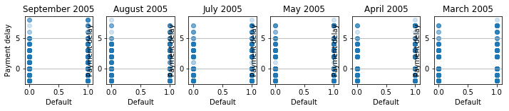
../_images/solution_2016_credit_clement_7_1.png

fig = plt.figure(figsize=(12, 6))
alpha=alpha_scatterplot = 0.2
alpha_bar_chart = 0.55

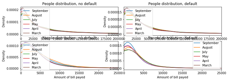
'''Graphs - bill statement'''

# personnes pas en défaut de paiement
ax1 = plt.subplot2grid((3,6),(1,0), colspan=3)
# kernel density
df1.X12[df1.Y == 0].plot(kind='kde')
df1.X13[df1.Y == 0].plot(kind='kde')
df1.X14[df1.Y == 0].plot(kind='kde')
df1.X15[df1.Y == 0].plot(kind='kde')
df1.X16[df1.Y == 0].plot(kind='kde')
df1.X17[df1.Y == 0].plot(kind='kde')
# axes
plt.xlabel("Bill statement")
plt.title("People distribution, no default")
# limites
ax1.set_xlim(0, 200000)
# légende
plt.legend(('September','August','July','May','April','March'),loc='best')

# personnes en défaut de paiement
ax2 = plt.subplot2grid((3,6),(1,3), colspan=3)
# kernel density
df1.X12[df1.Y == 1].plot(kind='kde')
df1.X13[df1.Y == 1].plot(kind='kde')
df1.X14[df1.Y == 1].plot(kind='kde')
df1.X15[df1.Y == 1].plot(kind='kde')
df1.X16[df1.Y == 1].plot(kind='kde')
df1.X17[df1.Y == 1].plot(kind='kde')
# axes
plt.xlabel("Bill statement")
plt.title("People distribution, default")
# limites
ax2.set_xlim(0, 200000)
# légende
plt.legend(('September','August','July','May','April','March'),loc='best')


'''Graphs - amount of bill payed'''

# personnes pas en défaut de paiement
ax1 = plt.subplot2grid((3,6),(2,0), colspan=3)
# kernel density
df1.X18[df1.Y == 0].plot(kind='kde')
df1.X19[df1.Y == 0].plot(kind='kde')
df1.X20[df1.Y == 0].plot(kind='kde')
df1.X21[df1.Y == 0].plot(kind='kde')
df1.X22[df1.Y == 0].plot(kind='kde')
df1.X23[df1.Y == 0].plot(kind='kde')
# axes
plt.xlabel("Amount of bill payed")
plt.title("People distribution, no default")
# limites
ax1.set_xlim(0, 25000)
# légende
plt.legend(('September','August','July','May','April','March'),loc='best')

# personnes en défaut de paiement
ax2 = plt.subplot2grid((3,6),(2,3), colspan=3)
# kernel density
df1.X18[df1.Y == 1].plot(kind='kde')
df1.X19[df1.Y == 1].plot(kind='kde')
df1.X20[df1.Y == 1].plot(kind='kde')
df1.X21[df1.Y == 1].plot(kind='kde')
df1.X22[df1.Y == 1].plot(kind='kde')
df1.X23[df1.Y == 1].plot(kind='kde')
# axes
plt.xlabel("Amount of bill payed")
plt.title("People distribution, default")
# limites
ax2.set_xlim(0, 25000)
# légende
plt.legend(('September','August','July','May','April','March'),loc='best')

<matplotlib.legend.Legend at 0x2a5065c50b8>

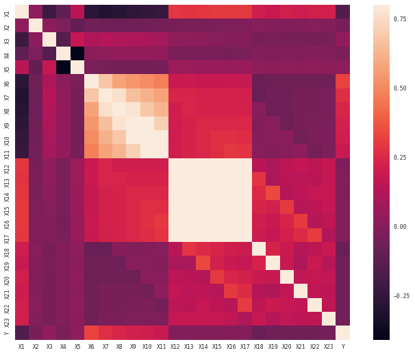
../_images/solution_2016_credit_clement_8_1.png

# Matrice des corrélations

sns.set(context="paper", font="monospace")
corrmat = df1.corr()

# atplotlib figure
f, ax = plt.subplots(figsize=(12, 9))

# Draw the heatmap using seaborn
sns.heatmap(corrmat, vmax=.8, square=True)

<matplotlib.axes._subplots.AxesSubplot at 0x2a506461588>

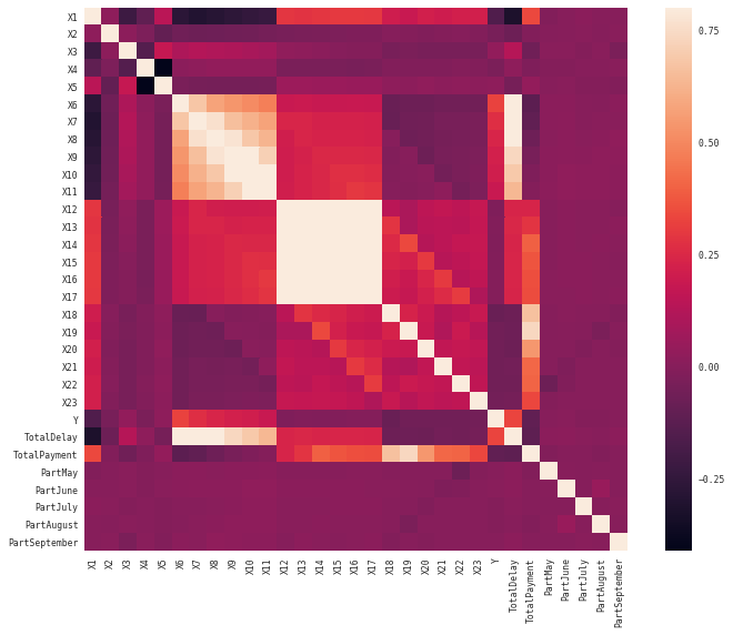
../_images/solution_2016_credit_clement_9_1.png

# on modifie les colonnes (création de variables d'intérêt)

df1['TotalDelay'] = df1.X11 + 2*df1.X10 + 4*df1.X9 + 8*df1.X8 + 16*df1.X7 + 32*df1.X6
df1['TotalPayment'] = df1.X23 + 2*df1.X22 + 3*df1.X21 + 4*df1.X20 + 5*df1.X19 + 6*df1.X18
df1['PartMay'] = -(df1.X22 - df1.X17)/(df1.X17 + 1)
df1['PartJune'] = -(df1.X21 - df1.X16)/(df1.X16 + 1)
df1['PartJuly'] = -(df1.X20 - df1.X15)/(df1.X15 + 1)
df1['PartAugust'] = -(df1.X19 - df1.X14)/(df1.X14 + 1)
df1['PartSeptember'] = -(df1.X18 - df1.X13)/(df1.X13 + 1)
df1.head(20)

	X1	X2	X3	X4	X5	X6	X7	X8	X9	X10	...	X22	X23	Y	TotalDelay	TotalPayment	PartMay	PartJune	PartJuly	PartAugust	PartSeptember
0	180000	1	2	1	47	0	0	0	0	0	...	2500	2618	0	0	71798	0.962902	0.964215	0.958865	0.961978	0.961112
1	110000	2	2	1	35	0	0	0	0	0	...	184	185	1	0	17094	0.963518	0.963962	0.777823	0.721906	0.850305
2	70000	2	2	2	22	0	0	0	0	0	...	1792	1793	1	0	51151	0.963766	0.964848	0.962690	0.956517	0.962942
3	200000	2	1	2	27	-2	-2	-2	-2	-2	...	0	95456	0	-126	224043	1.028571	-0.004450	-0.004802	-0.004502	-0.009899
4	370000	2	1	1	39	0	0	0	0	0	...	3000	1000	0	0	42614	0.937577	0.958029	0.965386	0.959245	0.968143
5	260000	2	1	1	29	0	0	0	-2	-2	...	0	141516	0	-14	160056	0.000000	0.000000	0.000000	0.000000	0.942813
6	90000	2	1	1	43	-1	-1	2	-1	-1	...	4009	7452	0	-39	135882	0.000000	0.000000	0.000000	0.997711	0.393333
7	220000	2	1	1	43	-1	3	2	0	0	...	0	0	1	32	1002	0.000000	0.999083	0.999083	0.999083	0.866455
8	50000	1	2	1	35	1	2	0	0	0	...	29935	1200	1	63	78530	-0.012172	0.985915	0.915291	0.956269	0.999979
9	50000	2	3	2	40	0	0	0	0	0	...	325	436	0	0	19283	0.962316	0.963619	0.879296	0.847636	0.806216
10	130000	1	2	1	24	0	0	2	0	0	...	0	780	0	16	38480	0.997442	0.999978	0.959249	0.999979	0.899013
11	200000	2	1	2	25	-1	-1	-1	-1	-1	...	4970	8888	0	-63	82748	0.000000	0.000000	0.000000	0.000000	0.000000
12	230000	2	2	1	38	-2	-2	-2	-2	-2	...	2132	2204	0	-126	111453	0.000000	0.000000	0.000000	0.000000	0.000000
13	90000	2	1	2	29	-2	-2	-2	-2	-2	...	0	0	0	-126	0	1.004184	1.004184	1.004184	1.004184	1.004184
14	230000	1	3	2	37	-1	0	0	0	-1	...	5003	3016	0	-34	287273	0.887873	-0.000340	0.769071	0.760863	0.952064
15	130000	1	2	2	33	2	2	-1	-1	-2	...	0	0	0	78	3578	0.000000	0.000000	0.000000	0.000000	0.993003
16	90000	2	2	1	35	0	0	0	0	0	...	4000	0	0	2	91108	0.954684	0.883510	0.952754	0.953646	0.952596
17	10000	2	2	1	37	-1	4	3	2	2	...	0	36	0	70	3236	0.999550	0.848221	0.800478	0.999590	0.999652
18	80000	1	3	1	36	0	0	0	0	0	...	3000	6200	0	0	73411	0.961214	0.926935	0.962670	0.963936	0.962893
19	320000	2	1	1	36	-1	2	0	0	0	...	5000	11906	0	0	96906	0.792507	0.755381	0.703680	0.400943	0.999851

20 rows × 31 columns

# Matrice des corrélations

sns.set(context="paper", font="monospace")
corrmat = df1.corr()

# matplotlib figure
f, ax = plt.subplots(figsize=(12, 9))

# Draw the heatmap using seaborn
sns.heatmap(corrmat, vmax=.8, square=True)

<matplotlib.axes._subplots.AxesSubplot at 0x2a5067c70f0>

../_images/solution_2016_credit_clement_11_1.png

# drop some columns

df1 = df1.drop(['X'+str(n) for n in range(7,12)] + ['X'+str(n) for n in range(13,24)], axis=1)
df1.head(20)

	X1	X2	X3	X4	X5	X6	X12	Y	TotalDelay	TotalPayment	PartMay	PartJune	PartJuly	PartAugust	PartSeptember
0	180000	1	2	1	47	0	179253	0	0	71798	0.962902	0.964215	0.958865	0.961978	0.961112
1	110000	2	2	1	35	0	6137	1	0	17094	0.963518	0.963962	0.777823	0.721906	0.850305
2	70000	2	2	2	22	0	66505	1	0	51151	0.963766	0.964848	0.962690	0.956517	0.962942
3	200000	2	1	2	27	-2	4941	0	-126	224043	1.028571	-0.004450	-0.004802	-0.004502	-0.009899
4	370000	2	1	1	39	0	141552	0	0	42614	0.937577	0.958029	0.965386	0.959245	0.968143
5	260000	2	1	1	29	0	71864	0	-14	160056	0.000000	0.000000	0.000000	0.000000	0.942813
6	90000	2	1	1	43	-1	16139	0	-39	135882	0.000000	0.000000	0.000000	0.997711	0.393333
7	220000	2	1	1	43	-1	1090	1	32	1002	0.000000	0.999083	0.999083	0.999083	0.866455
8	50000	1	2	1	35	1	48047	1	63	78530	-0.012172	0.985915	0.915291	0.956269	0.999979
9	50000	2	3	2	40	0	5538	0	0	19283	0.962316	0.963619	0.879296	0.847636	0.806216
10	130000	1	2	1	24	0	46113	0	16	38480	0.997442	0.999978	0.959249	0.999979	0.899013
11	200000	2	1	2	25	-1	8926	0	-63	82748	0.000000	0.000000	0.000000	0.000000	0.000000
12	230000	2	2	1	38	-2	12696	0	-126	111453	0.000000	0.000000	0.000000	0.000000	0.000000
13	90000	2	1	2	29	-2	-240	0	-126	0	1.004184	1.004184	1.004184	1.004184	1.004184
14	230000	1	3	2	37	-1	36571	0	-34	287273	0.887873	-0.000340	0.769071	0.760863	0.952064
15	130000	1	2	2	33	2	2183	0	78	3578	0.000000	0.000000	0.000000	0.000000	0.993003
16	90000	2	2	1	35	0	72112	0	2	91108	0.954684	0.883510	0.952754	0.953646	0.952596
17	10000	2	2	1	37	-1	3305	0	70	3236	0.999550	0.848221	0.800478	0.999590	0.999652
18	80000	1	3	1	36	0	81066	0	0	73411	0.961214	0.926935	0.962670	0.963936	0.962893
19	320000	2	1	1	36	-1	7868	0	0	96906	0.792507	0.755381	0.703680	0.400943	0.999851

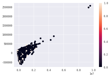
from sklearn.decomposition import PCA
from numpy import inf
pca = PCA(n_components=2, svd_solver='randomized')
dfpca = df1.values
dfpca[dfpca == -inf] = 0
y = dfpca[:, 7]
proj = pca.fit_transform(dfpca[:, :7 + 8:])
plt.scatter(proj[:, 0], proj[:, 1], c=y)
plt.colorbar()

<matplotlib.colorbar.Colorbar at 0x2a506a1a0b8>

../_images/solution_2016_credit_clement_13_1.png

# training/crossval set

X = df1.values
X[X==-inf] = 0
print(df1.head())
# training set
X_train = X[:, :]
Y_train = X[:, 7].ravel()
X_train = np.delete(X_train, 7, axis=1)
# expected result
expected = X[20000:, 7].ravel()
# cross-validation data set
X_cross = X[20000:, :]
X_cross = np.delete(X_cross, 7, axis=1)

       X1  X2  X3  X4  X5  X6     X12  Y  TotalDelay  TotalPayment   PartMay  0  180000   1   2   1  47   0  179253  0           0         71798  0.962902
1  110000   2   2   1  35   0    6137  1           0         17094  0.963518
2   70000   2   2   2  22   0   66505  1           0         51151  0.963766
3  200000   2   1   2  27  -2    4941  0        -126        224043  1.028571
4  370000   2   1   1  39   0  141552  0           0         42614  0.937577
   PartJune  PartJuly  PartAugust  PartSeptember
0  0.964215  0.958865    0.961978       0.961112
1  0.963962  0.777823    0.721906       0.850305
2  0.964848  0.962690    0.956517       0.962942
3 -0.004450 -0.004802   -0.004502      -0.009899
4  0.958029  0.965386    0.959245       0.968143

from sklearn.naive_bayes import GaussianNB

# train the model
GNB = GaussianNB()
GNB.fit(X_train, Y_train)

# use the model to predict the labels of the test data
predicted = GNB.predict(X_cross)

print(metrics.confusion_matrix(expected, predicted))

[[ 209 1732]
 [  26  533]]

from sklearn.ensemble import GradientBoostingClassifier

GBR = GradientBoostingClassifier()
GBR.fit(X_train,Y_train)
predicted = GBR.predict(X_cross)
print(metrics.confusion_matrix(expected, predicted))

[[1848   93]
 [ 352  207]]

from sklearn.neighbors import KNeighborsClassifier

KNC = KNeighborsClassifier(5)
KNC.fit(X_train, Y_train)
predicted = KNC.predict(X_cross)
print(metrics.confusion_matrix(expected, predicted))
pred = KNC.predict_proba(X_train)

[[1864   77]
 [ 368  191]]

print(pred[:10])
print(Y_train[:10])

[[ 1.   0. ]
 [ 0.6  0.4]
 [ 0.6  0.4]
 [ 1.   0. ]
 [ 1.   0. ]
 [ 0.6  0.4]
 [ 1.   0. ]
 [ 0.4  0.6]
 [ 0.4  0.6]
 [ 0.8  0.2]]
[ 0.  1.  1.  0.  0.  0.  0.  1.  1.  0.]

# neural network

from sklearn.neural_network import MLPClassifier
from sklearn.metrics import r2_score
from sklearn.model_selection import GridSearchCV

# optimisation - choix du nombre de couches
param_grid = [
  {'hidden_layer_sizes': [(nb,) for nb in range(20,50,10)]},
  {'alpha': [a/100 for a in range(0,40,20)]}
 ]

neural2 = GridSearchCV(MLPClassifier(), param_grid, verbose=1)
neural2.fit(X_train, Y_train)
neural2.best_estimator_

Fitting 3 folds for each of 5 candidates, totalling 15 fits

[Parallel(n_jobs=1)]: Done  15 out of  15 | elapsed:   27.2s finished

MLPClassifier(activation='relu', alpha=0.0001, batch_size='auto', beta_1=0.9,
       beta_2=0.999, early_stopping=False, epsilon=1e-08,
       hidden_layer_sizes=(20,), learning_rate='constant',
       learning_rate_init=0.001, max_iter=200, momentum=0.9,
       nesterovs_momentum=True, power_t=0.5, random_state=None,
       shuffle=True, solver='adam', tol=0.0001, validation_fraction=0.1,
       verbose=False, warm_start=False)

neural = MLPClassifier(activation='relu', alpha=0.0001, batch_size='auto', beta_1=0.9,
       beta_2=0.999, early_stopping=False, epsilon=1e-08,
       hidden_layer_sizes=(170,), learning_rate='constant',
       learning_rate_init=0.001, max_iter=200, momentum=0.9,
       nesterovs_momentum=True, power_t=0.5, random_state=None,
       shuffle=True, solver='adam', tol=0.0001, validation_fraction=0.1,
       verbose=False, warm_start=False)
neural.fit(X_train, Y_train)
predicted = neural.predict(X_cross)
print(metrics.confusion_matrix(expected, predicted))
neural.predict_proba(X_cross[:10])

[[1780  161]
 [ 378  181]]

array([[  1.00000000e+000,   4.54194423e-294],
       [  1.00000000e+000,   1.14673239e-101],
       [  1.00000000e+000,   1.13397258e-051],
       [  1.00000000e+000,   1.89540529e-117],
       [  1.00000000e+000,   8.01811448e-032],
       [  1.00000000e+000,   1.14003085e-160],
       [  1.00000000e+000,   1.02562443e-115],
       [  1.00000000e+000,   9.41507727e-017],
       [  1.00000000e+000,   3.16744761e-026],
       [  6.95744980e-001,   3.04255020e-001]])

if_you_have_time = False
if if_you_have_time:
    from sklearn.gaussian_process import GaussianProcessClassifier

    GPC = GaussianProcessClassifier()
    GPC.fit(X_train, Y_train)
    predicted = GPC.predict(X_cross)
    print(metrics.confusion_matrix(expected, predicted))
    GPC.predict_proba(X_cross)

from sklearn.ensemble import RandomForestClassifier

RFC = RandomForestClassifier(5)
RFC.fit(X_train, Y_train)
predicted = RFC.predict(X_cross)
print(metrics.confusion_matrix(expected, predicted))
print(RFC.predict_proba(X_cross))
print(expected)

[[1928   13]
 [  65  494]]
[[ 1.   0. ]
 [ 1.   0. ]
 [ 0.   1. ]
 ...,
 [ 1.   0. ]
 [ 1.   0. ]
 [ 0.8  0.2]]
[ 0.  0.  1. ...,  0.  0.  0.]

if if_you_have_time:
    from sklearn.svm import SVC

    SVC = SVC(probability = True)
    SVC.fit(X_train, Y_train)
    predicted = SVC.predict(X_cross)
    print(metrics.confusion_matrix(expected, predicted))
    print(SVC.predict_proba(X_cross))
    print(expected)

from sklearn.linear_model import LogisticRegression

LR = LogisticRegression()
LR.fit(X_train, Y_train)
predicted = LR.predict(X_cross)
print(metrics.confusion_matrix(expected, predicted))
print(LR.predict_proba(X_train))
print(Y_train)

[[1861   80]
 [ 413  146]]
[[ 0.85603222  0.14396778]
 [ 0.72020052  0.27979948]
 [ 0.69524708  0.30475292]
 ...,
 [ 0.69884026  0.30115974]
 [ 0.85309221  0.14690779]
 [ 0.75099513  0.24900487]]
[ 0.  1.  1. ...,  0.  0.  0.]

#--------------#
# modèle final #
#--------------#

# dataframe
dfend = pd.read_csv("ensae_competition_test_X.txt", header=[0, 1], sep='\t', encoding="utf8", index_col=0)
dfend.columns = dfend.columns.droplevel(-1)

# modifications colonnes
dfend['TotalDelay'] = dfend.X11 + 2*dfend.X10 + 4*dfend.X9 + 8*dfend.X8 + 16*dfend.X7 + 32*dfend.X6
dfend['TotalPayment'] = dfend.X23 + 2*dfend.X22 + 3*dfend.X21 + 4*dfend.X20 + 5*dfend.X19 + 6*dfend.X18
dfend['PartMay'] = -(dfend.X22 - dfend.X17)/(dfend.X17 + 1)
dfend['PartJune'] = -(dfend.X21 - dfend.X16)/(dfend.X16 + 1)
dfend['PartJuly'] = -(dfend.X20 - dfend.X15)/(dfend.X15 + 1)
dfend['PartAugust'] = -(dfend.X19 - dfend.X14)/(dfend.X14 + 1)
dfend['PartSeptember'] = -(dfend.X18 - dfend.X13)/(dfend.X13 + 1)
dfend = dfend.drop(['X'+str(n) for n in range(7,12)] + ['X'+str(n) for n in range(13,24)], axis=1)

# dataset as array
X = dfend.values
X[X==-inf] = 0

# prédictions

# réseau de neuronnes
l = neural.predict(X)
text_file = open('answerN.txt','w')
for e in l:
    text_file.write(str(int(e)) + '\n')
text_file.close()

# random forest
l = RFC.predict(X)
text_file = open('answerRF.txt','w')
for e in l:
    text_file.write(str(int(e)) + '\n')
text_file.close()

Liens

Contenu

Information

Sujet précédent

Sujet suivant

2016 - Une solution à la compétition de machine learning 2A#