Machine Learning éthique#

Links: notebook, html, python, slides, GitHub

Ce notebook est inspiré de l’article FairTest: Discovering Unwarranted Associations in Data-Driven Applications et propose d’étudier une façon de vérifier qu’un modèle ou une métrique n’est pas biaisé par rapport à certains critères.

from jyquickhelper import add_notebook_menu
add_notebook_menu()

Principe #

Un problème de machine learning dans sa définition la plus simple consiste à prédire $Y$ en fonction de $I$ . On souhaite construire une fonction $f(I)$ qui s’approche le plus possible de $Y$ . On appelle $I$ l’ensemble des données utilisateurs ou user input et $f(I)$ la sortie du modèle ou output to users (O). On veut découvrir si la sortie du modèle est biaisée d’une façon non-éthique par rapport à des attributs dits protégés ou protected attributes (S) tels que l’origine éthnique ou le genre. On tient compte également du contexte, code postal, …) ou context attributes (X) et de variables explicative ou explanotory attributes (E). On a donc :

I : les variables en entrée du modèles,
O : la prédiction du modèle,
S : les attributs protégés, toute corrélation entre la sortie et ces attributs est indésirable,
X : le contexte (principalement le lieu géographique)
E : les variables explicatives (contraintes qualitification), la sortie est a priori corrélée avec ces attributs, de façon quasi prévisible mais cela reste éthique.

Un exemple. Supposons qu’on cherche à recommander un objet à la vente sur un site internet à partir des données de navigation de cette personne (I). Comme cette personne est identifiée, on peut savoir où elle habite (X), son origine éthnique (S) et son niveau d’étude (E). Le site lui recommande un livre de mathématiques (O). Est-ce que cette recommandation dépend principalement de l’origine éthnique (S) ? Et si les deux informations semblent corrélées, ne serait-ce pas plutôt son niveau d’étude (E) qui explique la recommandation ?

Concrètement, la sortie O ne dépend que de I mais on souhaite savoir si I ne serait pas corrélées à certains facteurs qui ne sont pas éthique. C’est une corrélation inattendue mais observable. Le contexte X permet de partitionner et de vérifier si le modèle est éthique sur l’ensemble des sous-groupes de population. Le processus de recherche des corrélations indésirées s’effectue en cinq temps.

On choisit un attribut protégé $S_i$ et on réalise une partition de la population pour cet attribut.
On vérifie pour chaque sous-population (ou chaque partie) que la sortie O et l’attribut $S_i$ ne sont pas corrélés. C’est l’étape de détection.
Pour chaque biais détecté, on vérifie qu’il ne peut être expliqué par une des variables explicatrice auquel ce biais est acceptable. C’est l’étape de debugging.

%matplotlib inline

Installation de FairTest #

Le module ne peut pas être installé tel quel car il a été implémenté pour Python 2. Voici un lien qui devrait vous permettre de l’installer pour Python 3 si vous ne l’avez pas déjà fait.

# !pip install https://github.com/sdpython/fairtest/releases/download/0.1/fairtest-0.1-py3-none-any.whl

Données #

On récupère les données adult pour lequel il faut prédire le fait qu’une personne ait un revenu supérieur à 50.000 dollars par an.

import pyensae.datasource as ds
data = ds.download_data("adult.data",
                        url="https://archive.ics.uci.edu/ml/machine-learning-databases/adult/")
names = ("age,workclass,fnlwgt,education,education-num,marital-status,occupation,relationship,"
         "race,sexe,capital-gain,capital-loss,hours-per-week,native-country,income").split(",")

import pandas
df = pandas.read_csv(data, names=names)
df.head()

	age	workclass	fnlwgt	education	education-num	marital-status	occupation	relationship	race	sexe	capital-gain	hours-per-week	native-country	income
0	39	State-gov	77516	Bachelors	13	Never-married	Adm-clerical	Not-in-family	White	Male	2174	40	United-States	<=50K
1	50	Self-emp-not-inc	83311	Bachelors	13	Married-civ-spouse	Exec-managerial	Husband	White	Male	0	13	United-States	<=50K
2	38	Private	215646	HS-grad	9	Divorced	Handlers-cleaners	Not-in-family	White	Male	0	40	United-States	<=50K
3	53	Private	234721	11th	7	Married-civ-spouse	Handlers-cleaners	Husband	Black	Male	0	40	United-States	<=50K
4	28	Private	338409	Bachelors	13	Married-civ-spouse	Prof-specialty	Wife	Black	Female	0	40	Cuba	<=50K

Exemple avec aequitas #

aequitas propose un ensemble de métrique pour mesurer les biais éthiques.

from sklearn.model_selection import train_test_split
df2 = df.copy()
df2_train, df2_test = train_test_split(df2)

import numpy
label = "income"
X_train = df2_train.drop(label, axis=1)
y_train = df2_train[label] == ' >50K'
y_train = pandas.Series(numpy.array([1.0 if y else 0.0 for y in y_train]))
X_test = df2_test.drop(label, axis=1)
y_test = df2_test[label] == ' >50K'
y_test = pandas.Series(numpy.array([1.0 if y else 0.0 for y in y_test]))

X_train = X_train.drop(['fnlwgt'], axis=1).copy()
X_test = X_test.drop(['fnlwgt'], axis=1).copy()

cat_col = list(_ for _ in X_train.select_dtypes("object").columns)
cat_col

['workclass',
 'education',
 'marital-status',
 'occupation',
 'relationship',
 'race',
 'sexe',
 'native-country']

from sklearn.tree import DecisionTreeClassifier
from sklearn.pipeline import make_pipeline
from sklearn.preprocessing import LabelEncoder, OneHotEncoder



pipe = make_pipeline(
            OneHotEncoder(handle_unknown="ignore"),
            DecisionTreeClassifier(min_samples_leaf=10))
pipe.fit(X_train, y_train)

Pipeline(memory=None,
         steps=[('onehotencoder',
                 OneHotEncoder(categories='auto', drop=None,
                               dtype=<class 'numpy.float64'>,
                               handle_unknown='ignore', sparse=True)),
                ('decisiontreeclassifier',
                 DecisionTreeClassifier(ccp_alpha=0.0, class_weight=None,
                                        criterion='gini', max_depth=None,
                                        max_features=None, max_leaf_nodes=None,
                                        min_impurity_decrease=0.0,
                                        min_impurity_split=None,
                                        min_samples_leaf=10,
                                        min_samples_split=2,
                                        min_weight_fraction_leaf=0.0,
                                        presort='deprecated', random_state=None,
                                        splitter='best'))],
         verbose=False)

data = X_test.copy().reset_index(drop=True)
data["score"] = pipe.predict_proba(X_test)[:, 1]
data["label_value"] = y_test
data.head(n=4)

	age	workclass	education	education-num	marital-status	occupation	relationship	race	sexe	capital-gain	hours-per-week	native-country	score	label_value
0	38	Private	Some-college	10	Separated	Other-service	Not-in-family	White	Female	4650	72	United-States	0.000000	0.0
1	18	Private	HS-grad	9	Never-married	Sales	Own-child	White	Male	0	20	United-States	0.000000	0.0
2	44	Private	Some-college	10	Married-civ-spouse	Craft-repair	Husband	White	Male	0	60	United-States	0.500000	1.0
3	34	Private	HS-grad	9	Married-civ-spouse	Craft-repair	Husband	White	Male	0	40	United-States	0.333333	0.0

data_small = data[["sexe", "education", "score", "label_value"]].copy()
data_small.head(n=5)

	sexe	education	score	label_value
0	Female	Some-college	0.000000	0.0
1	Male	HS-grad	0.000000	0.0
2	Male	Some-college	0.500000	1.0
3	Male	HS-grad	0.333333	0.0
4	Male	HS-grad	0.000000	0.0

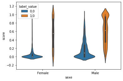
from seaborn import catplot, violinplot
g = violinplot(x="sexe", y="score", hue="label_value", data=data_small)

from aequitas.group import Group
g = Group()
xtab, _ = g.get_crosstabs(data_small)

model_id, score_thresholds 1 {'rank_abs': [472]}

xtab

	model_id	score_threshold	k	attribute_name	attribute_value	tpr	tnr	for	fdr	fpr	...	pprev	fp	fn	tn	tp	group_label_pos	group_label_neg	group_size	total_entities	prev
0	1	binary 0/1	472	sexe	Female	0.230769	0.999184	0.085821	0.028169	0.000816	...	0.025809	2	230	2450	69	299	2452	2751	8141	0.108688
1	1	binary 0/1	472	sexe	Male	0.243094	0.998671	0.247144	0.012469	0.001329	...	0.074397	5	1233	3756	396	1629	3761	5390	8141	0.302226
2	1	binary 0/1	472	education	10th	0.181818	1.000000	0.037975	0.000000	0.000000	...	0.008368	0	9	228	2	11	228	239	8141	0.046025
3	1	binary 0/1	472	education	11th	0.222222	1.000000	0.043210	0.000000	0.000000	...	0.012195	0	14	310	4	18	310	328	8141	0.054878
4	1	binary 0/1	472	education	12th	0.272727	1.000000	0.085106	0.000000	0.000000	...	0.030928	0	8	86	3	11	86	97	8141	0.113402
5	1	binary 0/1	472	education	1st-4th	0.000000	1.000000	0.068182	NaN	0.000000	...	0.000000	0	3	41	0	3	41	44	8141	0.068182
6	1	binary 0/1	472	education	5th-6th	0.000000	1.000000	0.040816	NaN	0.000000	...	0.000000	0	4	94	0	4	94	98	8141	0.040816
7	1	binary 0/1	472	education	7th-8th	0.100000	1.000000	0.056250	0.000000	0.000000	...	0.006211	0	9	151	1	10	151	161	8141	0.062112
8	1	binary 0/1	472	education	9th	0.000000	1.000000	0.045802	NaN	0.000000	...	0.000000	0	6	125	0	6	125	131	8141	0.045802
9	1	binary 0/1	472	education	Assoc-acdm	0.250000	1.000000	0.193966	0.000000	0.000000	...	0.060729	0	45	187	15	60	187	247	8141	0.242915
10	1	binary 0/1	472	education	Assoc-voc	0.185185	1.000000	0.217105	0.000000	0.000000	...	0.047022	0	66	238	15	81	238	319	8141	0.253918
11	1	binary 0/1	472	education	Bachelors	0.284173	0.998729	0.336149	0.006289	0.001271	...	0.118392	1	398	786	158	556	787	1343	8141	0.413999
12	1	binary 0/1	472	education	Doctorate	0.266667	0.950000	0.743243	0.047619	0.050000	...	0.221053	1	55	19	20	75	20	95	8141	0.789474
13	1	binary 0/1	472	education	HS-grad	0.165394	0.999557	0.126837	0.015152	0.000443	...	0.024887	1	328	2258	65	393	2259	2652	8141	0.148190
14	1	binary 0/1	472	education	Masters	0.317391	0.984536	0.451149	0.039474	0.015464	...	0.179245	3	157	191	73	230	194	424	8141	0.542453
15	1	binary 0/1	472	education	Preschool	NaN	1.000000	0.000000	NaN	0.000000	...	0.000000	0	0	17	0	0	17	17	8141	0.000000
16	1	binary 0/1	472	education	Prof-school	0.417476	0.971429	0.638298	0.022727	0.028571	...	0.318841	1	60	34	43	103	35	138	8141	0.746377
17	1	binary 0/1	472	education	Some-college	0.179837	1.000000	0.172790	0.000000	0.000000	...	0.036504	0	301	1441	66	367	1441	1808	8141	0.202987

18 rows × 26 columns

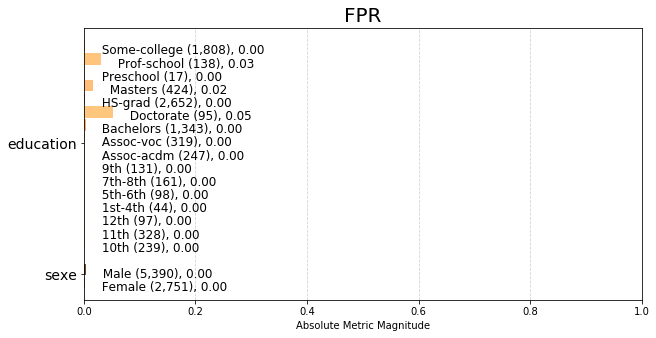
from aequitas.plotting import Plot

aqp = Plot()
fpr_plot = aqp.plot_group_metric(xtab, 'fpr')

set(data_small['education'])

{' 10th',
 ' 11th',
 ' 12th',
 ' 1st-4th',
 ' 5th-6th',
 ' 7th-8th',
 ' 9th',
 ' Assoc-acdm',
 ' Assoc-voc',
 ' Bachelors',
 ' Doctorate',
 ' HS-grad',
 ' Masters',
 ' Preschool',
 ' Prof-school',
 ' Some-college'}

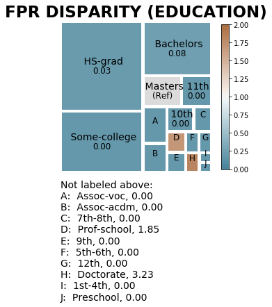
from aequitas.bias import Bias

b = Bias()
bdf = b.get_disparity_predefined_groups(xtab,
                    original_df=data_small,
                    ref_groups_dict={'sexe': ' Male', 'education':' Masters'},
                    alpha=0.05,
                    check_significance=False)

get_disparity_predefined_group()

fpr_disparity = aqp.plot_disparity(bdf, group_metric='fpr_disparity',
                                   attribute_name='education')

Exemple avec fairtest #

Ne fonctionne pas encore. Il faut passer à Python trois.

try:
    from fairtest import DataSource
    cont = True
except ImportError:
    cont = False
# On prend les 1000 premières lignes.
# Le processus est assez long.
if cont:
    dsdat = DataSource(df[:1000], budget=1, conf=0.95)

if cont:
    from fairtest import Testing, train, test, report

    SENS = ['sex', 'race']     # Protected features
    TARGET = 'income'             # Output
    EXPL = ''                     # Explanatory feature

    inv = Testing(dsdat, SENS, TARGET, EXPL)
    train([inv])

if cont:
    test([inv])

if cont:
    try:
        report([inv], "adult")
    except Exception as e:
        print("ERROR")
        print(e)
        # à corriger encore

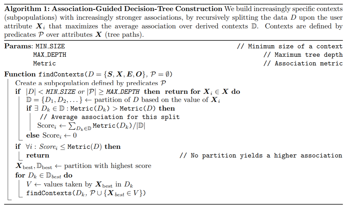
Exercice 1 : Construire un arbre de décision avec son propre critère #

On pourra s’inspirer de l’article Pure Python Decision Trees, ou How To Implement The Decision Tree Algorithm From Scratch In Python. Cet arbre de décision doit produire un résultat similaire à ceci : Contexte-education-num-in-(9.5, 11.5)-age-in(46.5, inf). Il s’agit d’implémenter l’algorithme qui suit avec la métrique Mutual Information (MI).

from pyquickhelper.helpgen import NbImage
NbImage("fairtesttree.png")

Exercice 2 : appliquer l’algorithme sur le jeu de données adulte #

Exercice 3 : apprendre sans interactions #

df2 = df.copy()
df2["un"] = 1
df2["age10"] = (df["age"] // 10) * 10
gr = df2[["age10", "sexe", "income", "un"]].groupby(["age10", "sexe", "income"], as_index=False).sum()
gr.head()

	age10	sexe	income	un
0	10	Female	<=50K	809
1	10	Female	>50K	1
2	10	Male	<=50K	846
3	10	Male	>50K	1
4	20	Female	<=50K	3048

g = gr.pivot_table("un", "age10", ["income", "sexe"])
g

income	<=50K		>50K
sexe	Female	Male	Female	Male
age10
10	809.0	846.0	1.0	1.0
20	3048.0	4497.0	128.0	381.0
30	2185.0	4119.0	391.0	1918.0
40	1778.0	2735.0	383.0	2279.0
50	1020.0	1691.0	207.0	1500.0
60	554.0	922.0	58.0	481.0
70	162.0	249.0	9.0	88.0
80	24.0	46.0	NaN	8.0
90	12.0	23.0	2.0	6.0

g.columns

MultiIndex([(' <=50K', ' Female'),
            (' <=50K',   ' Male'),
            ( ' >50K', ' Female'),
            ( ' >50K',   ' Male')],
           names=['income', 'sexe'])

g["rF"] = g[(" <=50K", " Female")] / g[(" >50K", " Female")]
g["rM"] = g[(" <=50K", " Male")] / g[(" >50K", " Male")]
g

income	<=50K		>50K		rF	rM
sexe	Female	Male	Female	Male
age10
10	809.0	846.0	1.0	1.0	809.000000	846.000000
20	3048.0	4497.0	128.0	381.0	23.812500	11.803150
30	2185.0	4119.0	391.0	1918.0	5.588235	2.147550
40	1778.0	2735.0	383.0	2279.0	4.642298	1.200088
50	1020.0	1691.0	207.0	1500.0	4.927536	1.127333
60	554.0	922.0	58.0	481.0	9.551724	1.916840
70	162.0	249.0	9.0	88.0	18.000000	2.829545
80	24.0	46.0	NaN	8.0	NaN	5.750000
90	12.0	23.0	2.0	6.0	6.000000	3.833333

Les deux variables paraissent corrélées.

On apprend trois modèles :

On prédit ‘income’ avec l’âge et le genre, modèle M0
On prédit ‘income’ avec l’âge uniquement, modèle M1
On prédit ‘income’ avec le genre uniquement, modèle M2
On prédit ‘income’ avec les modèles M1 et M2.

Le modèle prédit-il aussi bien, moins bien ? Qu’en déduisez-vous ?

Liens

Contenu

Information

Sujet précédent

Sujet suivant