datashader#
Links: notebook, html, PDF, python, slides, GitHub
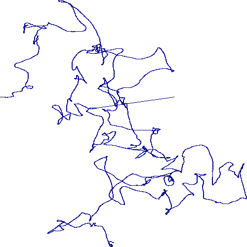
datashader plots huge volume of data.
from jyquickhelper import add_notebook_menu
add_notebook_menu()
import bokeh.plotting as bp
bp.output_notebook()
import datashader
datashader.__version__
'0.6.4dev1'
The version should be higher than 0.6.4.
short example#
From 4_Trajectories.ipynb.
import pandas as pd
import numpy as np
import xarray as xr
# On Windows, you must run the notebook with admin right
# otherwise the following instruction does not end.
import datashader
import datashader as ds
import datashader.transfer_functions as tf
# Constants
np.random.seed(1)
n = 1000000 # Number of points
f = filter_width = 5000 # momentum or smoothing parameter, for a moving average filter
# filtered random walk
xs = np.convolve(np.random.normal(0, 0.1, size=n), np.ones(f)/f).cumsum()
ys = np.convolve(np.random.normal(0, 0.1, size=n), np.ones(f)/f).cumsum()
# Add "mechanical" wobble on the x axis
xs += 0.1*np.sin(0.1*np.array(range(n-1+f)))
# Add "measurement" noise
xs += np.random.normal(0, 0.005, size=n-1+f)
ys += np.random.normal(0, 0.005, size=n-1+f)
# Add a completely incorrect value
xs[int(len(xs)/2)] = 100
ys[int(len(xs)/2)] = 0
# Create a dataframe
df = pd.DataFrame(dict(x=xs,y=ys))
# Default plot ranges:
x_range = (xs.min(), xs.max())
y_range = (ys.min(), ys.max())
df.tail()
| x | y | |
|---|---|---|
| 1004994 | 65.164829 | -105.064056 |
| 1004995 | 65.177603 | -105.069781 |
| 1004996 | 65.190898 | -105.071699 |
| 1004997 | 65.194054 | -105.054657 |
| 1004998 | 65.204752 | -105.073366 |
def create_image(x_range=x_range, y_range=y_range, w=500, h=500):
cvs = ds.Canvas(x_range=x_range, y_range=y_range, plot_height=h, plot_width=w)
agg = cvs.line(df, 'x', 'y', agg=ds.any())
return tf.shade(agg)
%time create_image()
Wall time: 1.1 s
from datashader.bokeh_ext import InteractiveImage
import bokeh.plotting as bp
def base_plot(tools='pan,wheel_zoom,reset'):
p = bp.figure(tools=tools, plot_width=500, plot_height=500,
x_range=x_range, y_range=y_range, outline_line_color=None,
min_border=0, min_border_left=0, min_border_right=0,
min_border_top=0, min_border_bottom=0)
p.xgrid.grid_line_color = None
p.ygrid.grid_line_color = None
return p
p = base_plot()
InteractiveImage(p, create_image)
NYC taxi#
without datashader#
import pandas as pd
import os
if os.path.exists('green_tripdata_2015-12.csv'):
df = pd.read_csv('green_tripdata_2015-12.csv',
usecols=['Pickup_longitude', 'Pickup_latitude',
'Dropoff_longitude', 'Dropoff_latitude',
'Passenger_count'])
df = df [(df.Dropoff_longitude < -10) & (df.Pickup_longitude < -10)]
df.sample(100000).to_csv("green_tripdata_2015-12_sample.csv")
else:
df = pd.read_csv("green_tripdata_2015-12_sample.csv")
df.tail()
| Unnamed: 0 | Pickup_longitude | Pickup_latitude | Dropoff_longitude | Dropoff_latitude | Passenger_count | |
|---|---|---|---|---|---|---|
| 99995 | 1505945 | -73.916512 | 40.777092 | -74.008743 | 40.704510 | 2 |
| 99996 | 968290 | -73.830383 | 40.759563 | -73.820259 | 40.751740 | 1 |
| 99997 | 1274687 | -73.899574 | 40.746056 | -73.899651 | 40.746105 | 2 |
| 99998 | 1023243 | -73.948578 | 40.789158 | -73.957741 | 40.776196 | 1 |
| 99999 | 261195 | -73.943939 | 40.711861 | -73.994743 | 40.684658 | 1 |
samples = df.sample(n=1000)
samples.head()
| Unnamed: 0 | Pickup_longitude | Pickup_latitude | Dropoff_longitude | Dropoff_latitude | Passenger_count | |
|---|---|---|---|---|---|---|
| 21828 | 824149 | -73.937645 | 40.679783 | -73.973488 | 40.680565 | 1 |
| 43531 | 622111 | -73.899452 | 40.743587 | -73.882927 | 40.741615 | 5 |
| 63837 | 291124 | -73.922501 | 40.708939 | -73.956100 | 40.688629 | 1 |
| 8116 | 1516644 | -73.995628 | 40.686577 | -73.986610 | 40.680191 | 1 |
| 73979 | 1283648 | -73.840294 | 40.695374 | -73.824905 | 40.706371 | 1 |
samples.describe()
| Unnamed: 0 | Pickup_longitude | Pickup_latitude | Dropoff_longitude | Dropoff_latitude | Passenger_count | |
|---|---|---|---|---|---|---|
| count | 1.000000e+03 | 1000.000000 | 1000.000000 | 1000.000000 | 1000.000000 | 1000.000000 |
| mean | 8.017301e+05 | -73.934097 | 40.745278 | -73.931417 | 40.741332 | 1.322000 |
| std | 4.551613e+05 | 0.044140 | 0.055953 | 0.051746 | 0.057068 | 0.946156 |
| min | 1.376000e+03 | -74.026848 | 40.587414 | -74.030685 | 40.578484 | 1.000000 |
| 25% | 4.124792e+05 | -73.960981 | 40.694023 | -73.965458 | 40.692575 | 1.000000 |
| 50% | 8.012435e+05 | -73.945271 | 40.742716 | -73.944492 | 40.742437 | 1.000000 |
| 75% | 1.206654e+06 | -73.914671 | 40.799161 | -73.904083 | 40.781639 | 1.000000 |
| max | 1.608100e+06 | -73.776367 | 40.887508 | -73.722435 | 40.909649 | 6.000000 |
from bokeh.plotting import figure, output_notebook, show
x_range=(samples.Dropoff_longitude.min(), samples.Dropoff_longitude.max())
y_range=(samples.Dropoff_latitude.min(), samples.Dropoff_latitude.max())
def base_plot(tools='pan,wheel_zoom,reset',plot_width=900, plot_height=600, **plot_args):
p = figure(tools=tools, plot_width=plot_width, plot_height=plot_height,
x_range=x_range, y_range=y_range, outline_line_color=None,
min_border=0, min_border_left=0, min_border_right=0,
min_border_top=0, min_border_bottom=0, **plot_args)
p.axis.visible = False
p.xgrid.grid_line_color = None
p.ygrid.grid_line_color = None
return p
from bokeh.tile_providers import STAMEN_TERRAIN, get_provider
p = base_plot()
tile_terrain = get_provider(STAMEN_TERRAIN)
p.add_tile(tile_terrain)
options = dict(line_color=None, fill_color='blue', size=5)
p.circle(x=samples['Dropoff_longitude'], y=samples['Dropoff_latitude'], **options)
show(p)
samples = df.sample(n=10000)
p = base_plot()
p.circle(x=samples['Dropoff_longitude'], y=samples['Dropoff_latitude'], **options)
show(p)
options = dict(line_color=None, fill_color='blue', size=1, alpha=0.1)
samples = df.sample(n=100000)
p = base_plot()
p.circle(x=samples['Dropoff_longitude'], y=samples['Dropoff_latitude'], **options)
show(p)
with datashader#
See nyc_taxi.ipynb. This part should be run with a bigger sample than the previous one.
import pandas as pd
import os
if os.path.exists('green_tripdata_2015-12.csv'):
df = pd.read_csv('green_tripdata_2015-12.csv',
usecols=['pickup_x', 'pickup_y', 'dropoff_x', 'dropoff_y',
'passenger_count', 'tpep_pickup_datetime'])
df = df [(df.dropoff_x < -10) & (df.dropoff_y < -10)]
df.sample(100000).to_csv("green_tripdata_2015-12_sample.csv")
else:
df = pd.read_csv("green_tripdata_2015-12_sample.csv")
df.columns = ['?', 'pickup_x', 'pickup_y', 'dropoff_x', 'dropoff_y',
'passenger_count']
df.tail()
| ? | pickup_x | pickup_y | dropoff_x | dropoff_y | passenger_count | |
|---|---|---|---|---|---|---|
| 99995 | 1505945 | -73.916512 | 40.777092 | -74.008743 | 40.704510 | 2 |
| 99996 | 968290 | -73.830383 | 40.759563 | -73.820259 | 40.751740 | 1 |
| 99997 | 1274687 | -73.899574 | 40.746056 | -73.899651 | 40.746105 | 2 |
| 99998 | 1023243 | -73.948578 | 40.789158 | -73.957741 | 40.776196 | 1 |
| 99999 | 261195 | -73.943939 | 40.711861 | -73.994743 | 40.684658 | 1 |
import datashader as ds
from datashader import transfer_functions as tf
from datashader.colors import Greys9
Greys9_r = list(reversed(Greys9))[:-2]
plot_width = int(750)
plot_height = int(plot_width//1.2)
cvs = ds.Canvas(plot_width=plot_width, plot_height=plot_height, x_range=x_range, y_range=y_range)
agg = cvs.points(df, 'dropoff_x', 'dropoff_y', ds.count('passenger_count'))
img = tf.shade(agg, cmap=["white", 'darkblue'], how='linear')
img
import numpy as np
def histogram(x,colors=None):
hist,edges = np.histogram(x, bins=100)
p = figure(y_axis_label="Pixels",
tools='', height=130, outline_line_color=None,
min_border=0, min_border_left=0, min_border_right=0,
min_border_top=0, min_border_bottom=0)
p.quad(top=hist[1:], bottom=0, left=edges[1:-1], right=edges[2:])
print("min: {}, max: {}".format(np.min(x),np.max(x)))
show(p)
histogram(agg.values)
min: 0, max: 175
histogram(np.log1p(agg.values))
tf.shade(agg, cmap=Greys9_r, how='log')
min: 0.0, max: 5.170483995038151
NYC = x_range, y_range = ((-8242000,-8210000), (4965000,4990000))
import datashader as ds
from datashader.bokeh_ext import InteractiveImage
from functools import partial
from datashader.utils import export_image
from datashader.colors import colormap_select, Greys9, Hot, viridis, inferno
from IPython.core.display import HTML, display
background = "black"
export = partial(export_image, export_path="export", background=background)
cm = partial(colormap_select, reverse=(background=="black"))
def create_image(x_range, y_range, w=plot_width, h=plot_height):
cvs = ds.Canvas(plot_width=w, plot_height=h, x_range=x_range, y_range=y_range)
agg = cvs.points(df, 'dropoff_x', 'dropoff_y', ds.count('passenger_count'))
img = tf.shade(agg, cmap=Hot, how='eq_hist')
return tf.dynspread(img, threshold=0.5, max_px=4)
p = base_plot(background_fill_color=background)
export(create_image(*NYC),"NYCT_hot")
InteractiveImage(p, create_image)
import numpy as np
from functools import partial
def create_image90(x_range, y_range, w=plot_width, h=plot_height):
cvs = ds.Canvas(plot_width=w, plot_height=h, x_range=x_range, y_range=y_range)
agg = cvs.points(df, 'dropoff_x', 'dropoff_y', ds.count('passenger_count'))
img = tf.shade(agg #.where(agg>np.percentile(agg,90)) # already a sample and it removes too many rows
, cmap=inferno, how='eq_hist')
return tf.dynspread(img, threshold=0.3, max_px=4)
p = base_plot()
p.add_tile(tile_terrain)
export(create_image(*NYC),"NYCT_90th")
InteractiveImage(p, create_image90)
def merged_images(x_range, y_range, w=plot_width, h=plot_height, how='log'):
cvs = ds.Canvas(plot_width=w, plot_height=h, x_range=x_range, y_range=y_range)
picks = cvs.points(df, 'pickup_x', 'pickup_y', ds.count('passenger_count'))
drops = cvs.points(df, 'dropoff_x', 'dropoff_y', ds.count('passenger_count'))
# already a sample and the following filter removes too many rows,
# you should use a bigger sample
more_drops = tf.shade(drops # .where(drops > picks)
, cmap=["darkblue", 'cornflowerblue'], how=how)
more_picks = tf.shade(picks # .where(picks > drops)
, cmap=["darkred", 'orangered'], how=how)
img = tf.stack(more_picks,more_drops)
return tf.dynspread(img, threshold=0.3, max_px=4)
p = base_plot(background_fill_color=background)
export(merged_images(*NYC),"NYCT_pickups_vs_dropoffs")
InteractiveImage(p, merged_images)