Deploy machine learned models with ONNX#
Links: notebook, html, PDF, python, slides, GitHub
Xavier Dupré - Senior Data Scientist at Microsoft - Computer Science Teacher at ENSAE
Most of machine learning libraries are optimized to train models and not necessarily to use them for fast predictions in online web services. ONNX is one solution started last year by Microsoft and Facebook. This presentation describes the concept and shows some examples with scikit-learn and ML.net.
La plupart des libraires de machine learning sont optimisées pour entraîner des modèles et pas nécessairement les utiliser dans des sites internet online où l’exigence de rapidité est importante. ONNX, une initiative open source proposée l’année dernière par Microsoft et Facebook est une réponse à ce problème. Ce talk illustrera ce concept avec un démo mêlant deep learning, scikit-learn et ML.net, la librairie de machine learning open source écrite en C# et développée par Microsoft.
from jyquickhelper import add_notebook_menu
add_notebook_menu(last_level=2)
from pyquickhelper.helpgen import NbImage
Open source tools in this talk#
import keras, lightgbm, onnx, skl2onnx, onnxruntime, sklearn, torch, xgboost
mods = [keras, lightgbm, onnx, skl2onnx, onnxruntime, sklearn, torch, xgboost]
for m in mods:
    print(m.__name__, m.__version__)
Using TensorFlow backend.
keras 2.3.1
lightgbm 2.3.1
onnx 1.7.105
skl2onnx 1.7.0
onnxruntime 1.3.993
sklearn 0.24.dev0
torch 1.5.0+cpu
xgboost 1.1.0
ML.net#
Open source in 2018
Machine learning library written in C#
Used in many places in Microsoft Services (Bing, …)
Working on it for three years
NbImage("mlnet.png", width=500)

onnx#
Serialisation library specialized for machine learning based on Google.Protobuf
Open source in 2017
NbImage("onnx.png", width=500)

sklearn-learn#
Open source in 2018
Converters for scikit-learn models
NbImage("sklearn-onnx.png")

onnxruntime#
Open source in December 2018
Available on Pypi/onnxruntime
documentation is here
source on microsoft/onnxruntime
Working on it for a couple of months
NbImage("onnxruntime.png", width=400)
Others tools#
The problem about deployment#
Learn and predict#
Two different purposes not necessarily aligned for optimization
Learn : computation optimized for large number of observations (batch prediction)
Predict : computation optimized for one observation (one-off prediction)
Machine learning libraries optimize the learn scenario.
Illustration with a linear regression#
We consider a datasets available in scikit-learn: diabetes
measures_lr = []
from sklearn.datasets import load_diabetes
diabetes = load_diabetes()
diabetes_X_train = diabetes.data[:-20]
diabetes_X_test  = diabetes.data[-20:]
diabetes_y_train = diabetes.target[:-20]
diabetes_y_test  = diabetes.target[-20:]
diabetes_X_train[:1]
array([[ 0.03807591,  0.05068012,  0.06169621,  0.02187235, -0.0442235 ,
        -0.03482076, -0.04340085, -0.00259226,  0.01990842, -0.01764613]])
scikit-learn#
from sklearn.linear_model import LinearRegression
clr = LinearRegression()
clr.fit(diabetes_X_train, diabetes_y_train)
LinearRegression()
clr.predict(diabetes_X_test[:1])
array([197.61846908])
from jupytalk.benchmark import timeexec
measures_lr += [timeexec("sklearn",
                         "clr.predict(diabetes_X_test[:1])",
                         context=globals())]
Average: 81.64 µs deviation 45.34 µs (with 50 runs) in [48.70 µs, 164.52 µs]
pure python#
def python_prediction(X, coef, intercept):
    s = intercept
    for a, b in zip(X, coef):
        s += a * b
    return s

python_prediction(diabetes_X_test[0], clr.coef_, clr.intercept_)
197.6184690750328
measures_lr += [timeexec("python",
                         "python_prediction(diabetes_X_test[0], clr.coef_, clr.intercept_)",
                         context=globals())]
Average: 12.53 µs deviation 9.88 µs (with 50 runs) in [5.92 µs, 28.09 µs]
Summary#
import pandas
df = pandas.DataFrame(data=measures_lr)
df = df.set_index("legend").sort_values("average")
df
| average | deviation | first | first3 | last3 | repeat | min5 | max5 | code | run | |
|---|---|---|---|---|---|---|---|---|---|---|
| legend | ||||||||||
| python | 0.000013 | 0.000010 | 0.000021 | 0.000015 | 0.000007 | 200 | 0.000006 | 0.000028 | python_prediction(diabetes_X_test[0], clr.coef... | 50 |
| sklearn | 0.000082 | 0.000045 | 0.000165 | 0.000139 | 0.000070 | 200 | 0.000049 | 0.000165 | clr.predict(diabetes_X_test[:1]) | 50 |
%matplotlib inline
import matplotlib.pyplot as plt
fig, ax = plt.subplots(1, 1, figsize=(10,3))
df[["average", "deviation"]].plot(kind="barh", logx=True, ax=ax, xerr="deviation",
                                  legend=False, fontsize=12, width=0.8)
ax.set_ylabel("")
ax.grid(b=True, which="major")
ax.grid(b=True, which="minor")
ax.set_title("Prediction time for one observation\nLinear Regression");
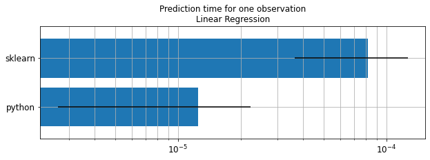
Illustration with a random forest#
measures_rf = []
scikit-learn#
from sklearn.ensemble import RandomForestRegressor
rf = RandomForestRegressor(n_estimators=10)
rf.fit(diabetes_X_train, diabetes_y_train)
RandomForestRegressor(n_estimators=10)
measures_rf += [timeexec("sklearn", "rf.predict(diabetes_X_test[:1])",
                         context=globals())]
Average: 1.01 ms deviation 155.50 µs (with 50 runs) in [852.33 µs, 1.37 ms]
XGBoost#
from xgboost import XGBRegressor
xg = XGBRegressor(n_estimators=10)
xg.fit(diabetes_X_train, diabetes_y_train)
XGBRegressor(base_score=0.5, booster='gbtree', colsample_bylevel=1,
             colsample_bynode=1, colsample_bytree=1, gamma=0, gpu_id=-1,
             importance_type='gain', interaction_constraints='',
             learning_rate=0.300000012, max_delta_step=0, max_depth=6,
             min_child_weight=1, missing=nan, monotone_constraints='()',
             n_estimators=10, n_jobs=0, num_parallel_tree=1, random_state=0,
             reg_alpha=0, reg_lambda=1, scale_pos_weight=1, subsample=1,
             tree_method='exact', validate_parameters=1, verbosity=None)
measures_rf += [timeexec("xgboost", "xg.predict(diabetes_X_test[:1])",
                         context=globals())]
Average: 1.48 ms deviation 322.72 µs (with 50 runs) in [1.18 ms, 2.23 ms]
LightGBM#
from lightgbm import LGBMRegressor
lg = LGBMRegressor(n_estimators=10)
lg.fit(diabetes_X_train, diabetes_y_train)
LGBMRegressor(n_estimators=10)
measures_rf += [timeexec("lightgbm", "lg.predict(diabetes_X_test[:1])",
                         context=globals())]
Average: 300.61 µs deviation 372.75 µs (with 50 runs) in [201.88 µs, 448.88 µs]
pure python#
This would require to reimplement the prediction function.
Summary#
df = pandas.DataFrame(data=measures_rf)
df = df.set_index("legend").sort_values("average")
df
| average | deviation | first | first3 | last3 | repeat | min5 | max5 | code | run | |
|---|---|---|---|---|---|---|---|---|---|---|
| legend | ||||||||||
| lightgbm | 0.000301 | 0.000373 | 0.000414 | 0.000333 | 0.000310 | 200 | 0.000202 | 0.000449 | lg.predict(diabetes_X_test[:1]) | 50 |
| sklearn | 0.001005 | 0.000156 | 0.001449 | 0.001280 | 0.000942 | 200 | 0.000852 | 0.001372 | rf.predict(diabetes_X_test[:1]) | 50 |
| xgboost | 0.001480 | 0.000323 | 0.001833 | 0.001643 | 0.001375 | 200 | 0.001178 | 0.002230 | xg.predict(diabetes_X_test[:1]) | 50 |
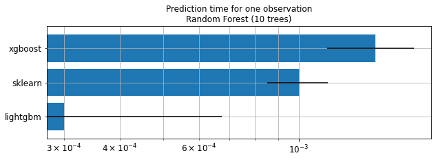
fig, ax = plt.subplots(1, 1, figsize=(10,3))
df[["average", "deviation"]].plot(kind="barh", logx=True, ax=ax, xerr="deviation",
                                  legend=False, fontsize=12, width=0.8)
ax.set_ylabel("")
ax.grid(b=True, which="major")
ax.grid(b=True, which="minor")
ax.set_title("Prediction time for one observation\nRandom Forest (10 trees)");
Keep in mind
Trained trees are not necessarily the same.
Performance is not compared.
Order of magnitude is important here.
What is batch prediction?#
Instead of running
 times 1 prediction
We run 1 time
predictions
import numpy
memo = []
batch = [1, 2, 5, 7, 8, 10, 100, 200, 500, 1000, 2000,
         3000, 4000, 5000, 10000, 20000, 50000,
         100000, 200000, 400000, ]

number = 10
repeat = 10
for i in batch:
    if i <= diabetes_X_test.shape[0]:
        mx = diabetes_X_test[:i]
    else:
        mxs = [diabetes_X_test] * (i // diabetes_X_test.shape[0] + 1)
        mx = numpy.vstack(mxs)
        mx = mx[:i]

    print("batch", "=", i)
    number = 10 if i <= 10000 else 2

    memo.append(timeexec("sklearn %d" % i, "rf.predict(mx)",
                         context=globals(), number=number, repeat=repeat))
    memo[-1]["batch"] = i
    memo[-1]["lib"] = "sklearn"

    memo.append(timeexec("xgboost %d" % i, "xg.predict(mx)",
                         context=globals(), number=number, repeat=repeat))
    memo[-1]["batch"] = i
    memo[-1]["lib"] = "xgboost"

    memo.append(timeexec("lightgbm %d" % i, "lg.predict(mx)",
                         context=globals(), number=number, repeat=repeat))
    memo[-1]["batch"] = i
    memo[-1]["lib"] = "lightgbm"
batch = 1
Average: 1.70 ms deviation 848.36 µs (with 10 runs) in [796.63 µs, 3.97 ms]
Average: 1.71 ms deviation 388.45 µs (with 10 runs) in [1.20 ms, 2.68 ms]
Average: 303.74 µs deviation 167.09 µs (with 10 runs) in [200.86 µs, 776.57 µs]
batch = 2
Average: 1.57 ms deviation 424.13 µs (with 10 runs) in [774.32 µs, 2.36 ms]
Average: 1.65 ms deviation 281.76 µs (with 10 runs) in [1.27 ms, 2.03 ms]
Average: 270.00 µs deviation 128.19 µs (with 10 runs) in [186.19 µs, 626.32 µs]
batch = 5
Average: 1.64 ms deviation 619.84 µs (with 10 runs) in [817.08 µs, 3.11 ms]
Average: 1.70 ms deviation 303.86 µs (with 10 runs) in [1.27 ms, 2.21 ms]
Average: 313.86 µs deviation 124.75 µs (with 10 runs) in [221.83 µs, 612.78 µs]
batch = 7
Average: 1.72 ms deviation 323.33 µs (with 10 runs) in [1.16 ms, 2.18 ms]
Average: 2.07 ms deviation 768.01 µs (with 10 runs) in [1.32 ms, 3.83 ms]
Average: 509.66 µs deviation 317.81 µs (with 10 runs) in [188.69 µs, 1.10 ms]
batch = 8
Average: 2.18 ms deviation 403.45 µs (with 10 runs) in [1.74 ms, 3.05 ms]
Average: 1.75 ms deviation 280.08 µs (with 10 runs) in [1.47 ms, 2.51 ms]
Average: 304.14 µs deviation 168.52 µs (with 10 runs) in [191.81 µs, 754.93 µs]
batch = 10
Average: 2.41 ms deviation 563.58 µs (with 10 runs) in [1.81 ms, 3.50 ms]
Average: 2.64 ms deviation 991.46 µs (with 10 runs) in [1.69 ms, 4.78 ms]
Average: 417.25 µs deviation 243.02 µs (with 10 runs) in [181.04 µs, 888.96 µs]
batch = 100
Average: 2.37 ms deviation 534.89 µs (with 10 runs) in [1.80 ms, 3.73 ms]
Average: 4.32 ms deviation 5.46 ms (with 10 runs) in [1.29 ms, 20.26 ms]
Average: 847.23 µs deviation 1.08 ms (with 10 runs) in [299.71 µs, 4.04 ms]
batch = 200
Average: 2.46 ms deviation 488.34 µs (with 10 runs) in [2.00 ms, 3.72 ms]
Average: 1.76 ms deviation 457.26 µs (with 10 runs) in [1.37 ms, 2.84 ms]
Average: 728.97 µs deviation 312.66 µs (with 10 runs) in [437.76 µs, 1.52 ms]
batch = 500
Average: 1.83 ms deviation 777.81 µs (with 10 runs) in [1.02 ms, 3.43 ms]
Average: 2.13 ms deviation 417.01 µs (with 10 runs) in [1.62 ms, 2.85 ms]
Average: 1.22 ms deviation 333.05 µs (with 10 runs) in [789.55 µs, 1.70 ms]
batch = 1000
Average: 2.76 ms deviation 1.71 ms (with 10 runs) in [1.43 ms, 7.76 ms]
Average: 2.00 ms deviation 323.80 µs (with 10 runs) in [1.45 ms, 2.59 ms]
Average: 2.22 ms deviation 1.01 ms (with 10 runs) in [1.41 ms, 4.44 ms]
batch = 2000
Average: 3.78 ms deviation 595.60 µs (with 10 runs) in [2.90 ms, 4.86 ms]
Average: 4.12 ms deviation 1.64 ms (with 10 runs) in [2.62 ms, 7.91 ms]
Average: 3.85 ms deviation 873.64 µs (with 10 runs) in [2.33 ms, 5.33 ms]
batch = 3000
Average: 3.78 ms deviation 695.73 µs (with 10 runs) in [2.94 ms, 4.87 ms]
Average: 5.42 ms deviation 3.44 ms (with 10 runs) in [3.19 ms, 14.98 ms]
Average: 4.04 ms deviation 875.18 µs (with 10 runs) in [2.83 ms, 5.51 ms]
batch = 4000
Average: 3.86 ms deviation 841.28 µs (with 10 runs) in [2.77 ms, 4.88 ms]
Average: 3.74 ms deviation 1.07 ms (with 10 runs) in [2.87 ms, 5.73 ms]
Average: 6.60 ms deviation 1.16 ms (with 10 runs) in [4.60 ms, 8.38 ms]
batch = 5000
Average: 4.61 ms deviation 776.78 µs (with 10 runs) in [3.62 ms, 6.33 ms]
Average: 4.11 ms deviation 499.51 µs (with 10 runs) in [3.54 ms, 4.98 ms]
Average: 6.91 ms deviation 3.28 ms (with 10 runs) in [4.52 ms, 15.27 ms]
batch = 10000
Average: 8.50 ms deviation 2.25 ms (with 10 runs) in [6.62 ms, 14.53 ms]
Average: 7.70 ms deviation 1.09 ms (with 10 runs) in [6.14 ms, 10.03 ms]
Average: 10.58 ms deviation 1.69 ms (with 10 runs) in [9.09 ms, 14.52 ms]
batch = 20000
Average: 15.31 ms deviation 2.15 ms (with 2 runs) in [12.73 ms, 18.75 ms]
Average: 15.86 ms deviation 6.96 ms (with 2 runs) in [11.53 ms, 35.46 ms]
Average: 24.20 ms deviation 6.72 ms (with 2 runs) in [16.32 ms, 36.71 ms]
batch = 50000
Average: 26.94 ms deviation 5.32 ms (with 2 runs) in [22.56 ms, 41.71 ms]
Average: 34.61 ms deviation 10.53 ms (with 2 runs) in [24.72 ms, 55.55 ms]
Average: 53.70 ms deviation 13.05 ms (with 2 runs) in [37.48 ms, 79.96 ms]
batch = 100000
Average: 53.32 ms deviation 6.81 ms (with 2 runs) in [46.19 ms, 66.79 ms]
Average: 71.28 ms deviation 5.78 ms (with 2 runs) in [63.42 ms, 81.72 ms]
Average: 88.06 ms deviation 13.45 ms (with 2 runs) in [74.47 ms, 112.05 ms]
batch = 200000
Average: 105.57 ms deviation 5.95 ms (with 2 runs) in [101.27 ms, 121.74 ms]
Average: 101.46 ms deviation 5.65 ms (with 2 runs) in [95.85 ms, 113.17 ms]
Average: 162.24 ms deviation 6.56 ms (with 2 runs) in [157.09 ms, 176.14 ms]
batch = 400000
Average: 203.91 ms deviation 20.09 ms (with 2 runs) in [192.94 ms, 263.38 ms]
Average: 196.82 ms deviation 11.00 ms (with 2 runs) in [184.06 ms, 218.61 ms]
Average: 303.72 ms deviation 12.70 ms (with 2 runs) in [285.54 ms, 328.46 ms]
dfb = pandas.DataFrame(memo)[["average", "lib", "batch"]]
piv = dfb.pivot("batch", "lib", "average")
for c in piv.columns:
piv["ave_" + c] = piv[c] / piv.index
libs = list(c for c in piv.columns if "ave_" in c)
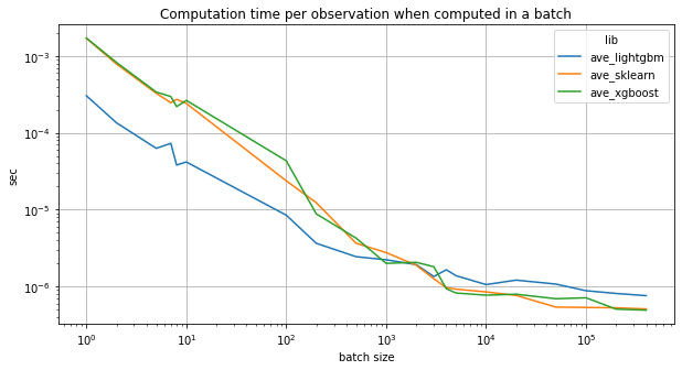
ax = piv.plot(y=libs, logy=True, logx=True, figsize=(10, 5))
ax.set_title("Computation time per observation when computed in a batch")
ax.set_ylabel("sec")
ax.set_xlabel("batch size")
ax.grid(True);
ONNX#
ONNX = language to describe models#
Standard format to describe machine learning
Easier to exchange, export
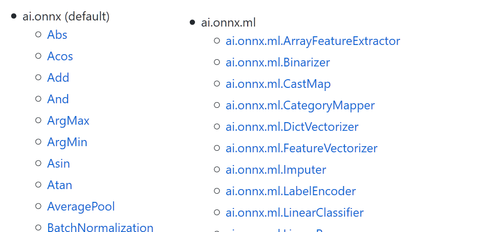
ONNX = machine learning oriented#
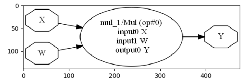
Can represent any mathematical function handling numerical and text features.
NbImage("onnxop.png", width=600)
ONNX = efficient serialization#
Based on google.protobuf
actively supported#
Microsoft
Facebook
first created to deploy deep learning models
extended to other models
Train somewhere, predict somewhere else#
Cannot optimize the code for both training and predicting.
Training |
Predicting |
|---|---|
Batch prediction |
One-off prediction |
Huge memory |
Small memory |
Huge data |
Small data |
. |
High latency |
Libraries for predictions#
Optimized for predictions
Optimized for a device
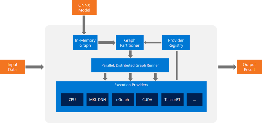
ONNX Runtime#
ONNX Runtime for inferencing machine learning models now in preview
Dedicated runtime for:
CPU
GPU
…
NbImage("onnxrt.png", width=800)
ONNX demo on random forest#
rf
RandomForestRegressor(n_estimators=10)
Conversion to ONNX#
onnxmltools
from skl2onnx import convert_sklearn
from skl2onnx.common.data_types import FloatTensorType
model_onnx = convert_sklearn(rf, "rf_diabetes",
                             [('input', FloatTensorType([1, 10]))])
print(str(model_onnx)[:450] + "\n...")
ir_version: 6
producer_name: "skl2onnx"
producer_version: "1.7.0"
domain: "ai.onnx"
model_version: 0
doc_string: ""
graph {
  node {
    input: "input"
    output: "variable"
    name: "TreeEnsembleRegressor"
    op_type: "TreeEnsembleRegressor"
    attribute {
      name: "n_targets"
      i: 1
      type: INT
    }
    attribute {
      name: "nodes_falsenodeids"
      ints: 282
      ints: 215
      ints: 212
      ints: 211
      ints: 104
...
Save the model#
def save_model(model, filename):
    with open(filename, "wb") as f:
        f.write(model.SerializeToString())

save_model(model_onnx, 'rf_sklearn.onnx')
Computes predictions#
import onnxruntime

sess = onnxruntime.InferenceSession("rf_sklearn.onnx")

for i in sess.get_inputs():
    print('Input:', i)
for o in sess.get_outputs():
    print('Output:', o)
Input: NodeArg(name='input', type='tensor(float)', shape=[1, 10])
Output: NodeArg(name='variable', type='tensor(float)', shape=[1, 1])
import numpy

def predict_onnxrt(x):
    return sess.run(["variable"], {'input': x})

print("Prediction:", predict_onnxrt(diabetes_X_test[:1].astype(numpy.float32)))
Prediction: [array([[223.9]], dtype=float32)]
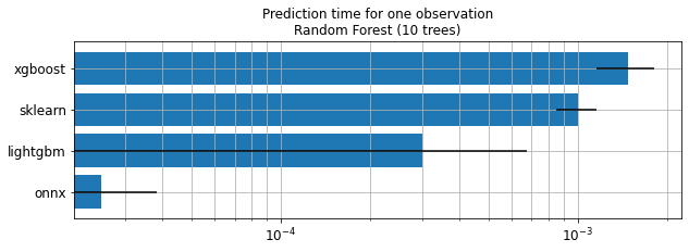
measures_rf += [timeexec("onnx", "predict_onnxrt(diabetes_X_test[:1].astype(numpy.float32))",
                         context=globals())]
Average: 24.95 µs deviation 13.21 µs (with 50 runs) in [14.63 µs, 53.23 µs]
fig, ax = plt.subplots(1, 1, figsize=(10,3))
df = pandas.DataFrame(data=measures_rf)
df = df.set_index("legend").sort_values("average")
df[["average", "deviation"]].plot(kind="barh", logx=True, ax=ax, xerr="deviation",
                                  legend=False, fontsize=12, width=0.8)
ax.set_ylabel("")
ax.grid(b=True, which="major")
ax.grid(b=True, which="minor")
ax.set_title("Prediction time for one observation\nRandom Forest (10 trees)");
Deep learning#
transfer learning with keras
orther convert pytorch, caffee…
measures_dl = []
from keras.applications.mobilenet_v2 import MobileNetV2
model = MobileNetV2(input_shape=None, alpha=1.0, include_top=True,
                    weights='imagenet', input_tensor=None,
                    pooling=None, classes=1000)
model
<keras.engine.training.Model at 0x1760cbdef28>
from pyensae.datasource import download_data
import os
if not os.path.exists("simages/noclass"):
    os.makedirs("simages/noclass")
images = download_data("dog-cat-pixabay.zip",
                       whereTo="simages/noclass")
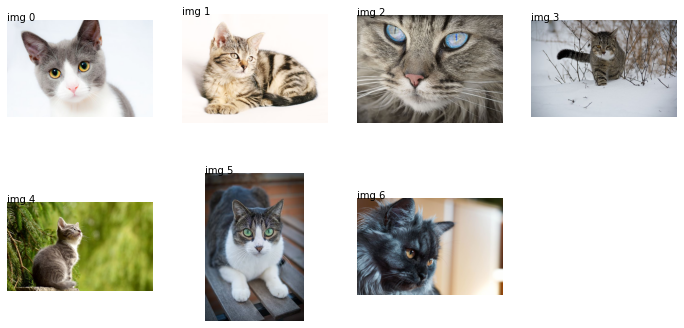
from mlinsights.plotting import plot_gallery_images
plot_gallery_images(images[:7]);
from keras.preprocessing.image import ImageDataGenerator
import numpy
params = dict(rescale=1./255)
augmenting_datagen = ImageDataGenerator(**params)
flow = augmenting_datagen.flow_from_directory('simages', batch_size=1, target_size=(224, 224),
                                              classes=['noclass'], shuffle=False)
imgs = [img[0][0] for i, img in zip(range(0,31), flow)]
Found 31 images belonging to 1 classes.
array_images = [im[numpy.newaxis, :, :, :] for im in imgs]
array_images[0].shape
(1, 224, 224, 3)
outputs = [model.predict(im) for im in array_images]
outputs[0].shape
(1, 1000)
outputs[0].ravel()[:10]
array([3.5999462e-04, 1.2039436e-03, 1.2471736e-04, 6.1937251e-05,
       1.1310312e-03, 1.7601081e-04, 1.9819051e-04, 1.4307769e-04,
       5.5190804e-04, 1.7074021e-04], dtype=float32)
Let’s measure time.
from jupytalk.benchmark import timeexec
measures_dl += [timeexec("mobilenet.keras", "model.predict(array_images[0])",
                         context=globals(), repeat=3, number=10)]
Average: 85.39 ms deviation 6.55 ms (with 10 runs) in [80.37 ms, 94.65 ms]
from keras2onnx import convert_keras
try:
    konnx = convert_keras(model, "mobilev2", target_opset=12)
except (ValueError, AttributeError) as e:
    # keras updated its version on
    print(e)
tf executing eager_mode: True
WARNING: Logging before flag parsing goes to stderr.
I0609 11:05:50.269349 34312 main.py:44] tf executing eager_mode: True
'tuple' object has no attribute 'layer'
Let’s switch to pytorch.
import torchvision.models as models
modelt = models.squeezenet1_1(pretrained=True)
modelt.classifier
Sequential(
  (0): Dropout(p=0.5, inplace=False)
  (1): Conv2d(512, 1000, kernel_size=(1, 1), stride=(1, 1))
  (2): ReLU(inplace=True)
  (3): AdaptiveAvgPool2d(output_size=(1, 1))
)
from torchvision import datasets, transforms
from torch.utils.data import DataLoader
trans = transforms.Compose([transforms.Resize((224, 224)),
                            transforms.CenterCrop(224),
                            transforms.ToTensor()])
imgs = datasets.ImageFolder("simages", trans)
dataloader = DataLoader(imgs, batch_size=1, shuffle=False, num_workers=1)
img_seq = iter(dataloader)
imgs = list(img[0] for img in img_seq)
all_outputs = [modelt.forward(img).detach().numpy().ravel() for img in imgs[:2]]
all_outputs[0].shape
(1000,)
measures_dl += [timeexec("squeezenet.pytorch", "modelt.forward(imgs[0]).detach().numpy().ravel()",
                         context=globals(), repeat=3, number=10)]
Average: 59.16 ms deviation 2.33 ms (with 10 runs) in [56.30 ms, 62.02 ms]
Let’s convert into ONNX.
import torch.onnx
from torch.autograd import Variable
input_names = [ "actual_input_1" ]
output_names = [ "output1" ]
dummy_input = Variable(torch.randn(1, 3, 224, 224))

torch.onnx.export(modelt, dummy_input, "squeezenet.torch.onnx", verbose=False,
                  input_names=input_names, output_names=output_names)
It works.
from onnxruntime import InferenceSession
sess = InferenceSession('squeezenet.torch.onnx')
inputs = [_.name for _ in sess.get_inputs()]
input_name = inputs[0]
input_name
'actual_input_1'
array_images[0].shape
(1, 224, 224, 3)
res = sess.run(None, {input_name: array_images[0].transpose((0, 3, 1, 2))})
res[0].shape
(1, 1000)
measures_dl += [timeexec("squeezenet.pytorch.onnx",
                         "sess.run(None, {input_name: array_images[0].transpose((0, 3, 1, 2))})",
                         context=globals(), repeat=3, number=10)]
Average: 10.21 ms deviation 1.55 ms (with 10 runs) in [8.20 ms, 11.96 ms]
Model zoo#
NbImage("zoo.png", width=800)
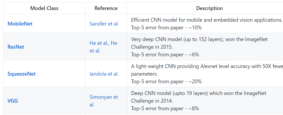
MobileNet and SqueezeNet#
Download a pre-converted version MobileNetv2
download_data("mobilenetv2-1.0.onnx",
              url="https://s3.amazonaws.com/onnx-model-zoo/mobilenet/mobilenetv2-1.0/")
'mobilenetv2-1.0.onnx'
sess = onnxruntime.InferenceSession("mobilenetv2-1.0.onnx")
for i in sess.get_inputs():
    print('Input:', i)
for o in sess.get_outputs():
    print('Output:', o)
Input: NodeArg(name='data', type='tensor(float)', shape=[1, 3, 224, 224])
Output: NodeArg(name='mobilenetv20_output_flatten0_reshape0', type='tensor(float)', shape=[1, 1000])
print(array_images[0].shape)
print(array_images[0].transpose((0, 3, 1, 2)).shape)
(1, 224, 224, 3)
(1, 3, 224, 224)
res = sess.run(None, {'data': array_images[0].transpose((0, 3, 1, 2))})
res[0].shape
(1, 1000)
measures_dl += [timeexec("mobile.zoo.onnx",
                         "sess.run(None, {'data': array_images[0].transpose((0, 3, 1, 2))})",
                         context=globals(), repeat=3, number=10)]
Average: 15.54 ms deviation 2.58 ms (with 10 runs) in [12.61 ms, 18.88 ms]
Download a pre-converted version SqueezeNet
download_data("squeezenet1.1.onnx",
              url="https://s3.amazonaws.com/onnx-model-zoo/squeezenet/squeezenet1.1/")
'squeezenet1.1.onnx'
sess = onnxruntime.InferenceSession("squeezenet1.1.onnx")
for i in sess.get_inputs():
    print('Input:', i)
for o in sess.get_outputs():
    print('Output:', o)
Input: NodeArg(name='data', type='tensor(float)', shape=[1, 3, 224, 224])
Output: NodeArg(name='squeezenet0_flatten0_reshape0', type='tensor(float)', shape=[1, 1000])
measures_dl += [timeexec("squeezenet.zoo.onnx",
                         "sess.run(None, {'data': array_images[0].transpose((0, 3, 1, 2))})",
                         context=globals(), repeat=3, number=10)]
Average: 13.43 ms deviation 2.10 ms (with 10 runs) in [11.26 ms, 16.28 ms]
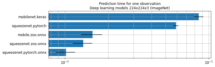
fig, ax = plt.subplots(1, 1, figsize=(10,3))
df = pandas.DataFrame(data=measures_dl)
df = df.set_index("legend").sort_values("average")
df[["average", "deviation"]].plot(kind="barh", logx=True, ax=ax, xerr="deviation",
                                  legend=False, fontsize=12, width=0.8)
ax.set_ylabel("")
ax.grid(b=True, which="major")
ax.grid(b=True, which="minor")
ax.set_title("Prediction time for one observation\nDeep learning models 224x224x3 (ImageNet)");
Tiny yolo#
Source: TinyYOLOv2 on onnx
download_data("tiny_yolov2.tar.gz",
              url="https://onnxzoo.blob.core.windows.net/models/opset_8/tiny_yolov2/")
['.\tiny_yolov2/./Model.onnx',
 '.\tiny_yolov2/./test_data_set_2/input_0.pb',
 '.\tiny_yolov2/./test_data_set_2/output_0.pb',
 '.\tiny_yolov2/./test_data_set_1/input_0.pb',
 '.\tiny_yolov2/./test_data_set_1/output_0.pb',
 '.\tiny_yolov2/./test_data_set_0/input_0.pb',
 '.\tiny_yolov2/./test_data_set_0/output_0.pb']
sess = onnxruntime.InferenceSession("tiny_yolov2/Model.onnx")
for i in sess.get_inputs():
    print('Input:', i)
for o in sess.get_outputs():
    print('Output:', o)
Input: NodeArg(name='image', type='tensor(float)', shape=['None', 3, 416, 416])
Output: NodeArg(name='grid', type='tensor(float)', shape=['None', 125, 13, 13])
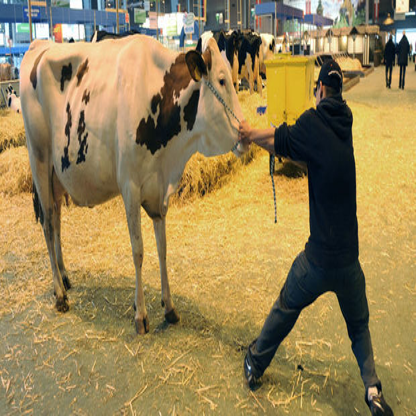
from PIL import Image,ImageDraw
img = Image.open('Au-Salon-de-l-agriculture-la-campagne-recrute.jpg')
img

img2 = img.resize((416, 416))
img2
X = numpy.asarray(img2)
X = X.transpose(2,0,1)
X = X.reshape(1,3,416,416)

out = sess.run(None, {'image': X.astype(numpy.float32)})
out = out[0][0]
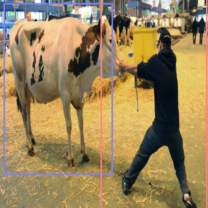
def display_yolo(img, seuil):
    import numpy as np
    numClasses = 20
    anchors = [1.08, 1.19, 3.42, 4.41, 6.63, 11.38, 9.42, 5.11, 16.62, 10.52]

    def sigmoid(x, derivative=False):
        return x*(1-x) if derivative else 1/(1+np.exp(-x))

    def softmax(x):
        scoreMatExp = np.exp(np.asarray(x))
        return scoreMatExp / scoreMatExp.sum(0)

    clut = [(0,0,0),(255,0,0),(255,0,255),(0,0,255),(0,255,0),(0,255,128),
            (128,255,0),(128,128,0),(0,128,255),(128,0,128),
            (255,0,128),(128,0,255),(255,128,128),(128,255,128),(255,255,0),
            (255,128,128),(128,128,255),(255,128,128),(128,255,128),(128,255,128)]
    label = ["aeroplane","bicycle","bird","boat","bottle",
             "bus","car","cat","chair","cow","diningtable",
             "dog","horse","motorbike","person","pottedplant",
             "sheep","sofa","train","tvmonitor"]

    draw = ImageDraw.Draw(img)
    for cy in range(0,13):
        for cx in range(0,13):
            for b in range(0,5):
                channel = b*(numClasses+5)
                tx = out[channel  ][cy][cx]
                ty = out[channel+1][cy][cx]
                tw = out[channel+2][cy][cx]
                th = out[channel+3][cy][cx]
                tc = out[channel+4][cy][cx]

                x = (float(cx) + sigmoid(tx))*32
                y = (float(cy) + sigmoid(ty))*32

                w = np.exp(tw) * 32 * anchors[2*b  ]
                h = np.exp(th) * 32 * anchors[2*b+1]

                confidence = sigmoid(tc)

                classes = np.zeros(numClasses)
                for c in range(0,numClasses):
                    classes[c] = out[channel + 5 +c][cy][cx]
                    classes = softmax(classes)
                detectedClass = classes.argmax()

                if seuil < classes[detectedClass]*confidence:
                    color =clut[detectedClass]
                    x = x - w/2
                    y = y - h/2
                    draw.line((x  ,y  ,x+w,y ),fill=color, width=3)
                    draw.line((x  ,y  ,x  ,y+h),fill=color, width=3)
                    draw.line((x+w,y  ,x+w,y+h),fill=color, width=3)
                    draw.line((x  ,y+h,x+w,y+h),fill=color, width=3)

    return img
img2 = img.resize((416, 416))
display_yolo(img2, 0.038)
Conclusion#
ONNX is a working progress, active development
ONNX is open source
ONNX does not depend on the machine learning framework
ONNX provides dedicated runtimes
ONNX is fast, available in Python…
Metadata to trace deployed models
meta = sess.get_modelmeta()
meta.description
"The Tiny YOLO network from the paper 'YOLO9000: Better, Faster, Stronger' (2016), arXiv:1612.08242"
meta.producer_name, meta.version
('OnnxMLTools', 0)