Faster Polynomial Features#

Links: notebook, html, PDF, python, slides, GitHub

from jyquickhelper import add_notebook_menu
add_notebook_menu()

%matplotlib inline

Polynomial Features #

The current implementation of PolynomialFeatures (0.20.2) implements a term by term product for each pair $X_i, X_j$ of features where $i \leqslant j$ which is not the most efficient way to do it.

import numpy.random
X = numpy.random.random((100, 5))

from sklearn.preprocessing import PolynomialFeatures
poly = PolynomialFeatures(degree=2)
Xpoly = poly.fit_transform(X)
poly.get_feature_names()

['1',
 'x0',
 'x1',
 'x2',
 'x3',
 'x4',
 'x0^2',
 'x0 x1',
 'x0 x2',
 'x0 x3',
 'x0 x4',
 'x1^2',
 'x1 x2',
 'x1 x3',
 'x1 x4',
 'x2^2',
 'x2 x3',
 'x2 x4',
 'x3^2',
 'x3 x4',
 'x4^2']

%timeit poly.transform(X)

114 µs ± 12.4 µs per loop (mean ± std. dev. of 7 runs, 10000 loops each)

The class ExtendedFeatures implements a different way to compute the polynomial features as it tries to reduce the number of calls to numpy by using broacasted vector multplications.

from mlinsights.mlmodel import ExtendedFeatures
ext = ExtendedFeatures(poly_degree=2)
Xpoly = ext.fit_transform(X)
ext.get_feature_names()

['1',
 'x0',
 'x1',
 'x2',
 'x3',
 'x4',
 'x0^2',
 'x0 x1',
 'x0 x2',
 'x0 x3',
 'x0 x4',
 'x1^2',
 'x1 x2',
 'x1 x3',
 'x1 x4',
 'x2^2',
 'x2 x3',
 'x2 x4',
 'x3^2',
 'x3 x4',
 'x4^2']

%timeit ext.transform(X)

68.7 µs ± 10.6 µs per loop (mean ± std. dev. of 7 runs, 10000 loops each)

Comparison with 5 features #

from cpyquickhelper.numbers import measure_time

res = []
for n in [1, 2, 5, 10, 20, 50, 100, 200, 500, 1000, 2000,
          5000, 10000, 20000, 50000, 100000, 200000]:
    X = numpy.random.random((n, 5))
    poly.fit(X)
    ext.fit(X)
    r1 = measure_time("poly.transform(X)", context=dict(X=X, poly=poly), repeat=5, number=10, div_by_number=True)
    r2 = measure_time("ext.transform(X)", context=dict(X=X, ext=ext), repeat=5, number=10, div_by_number=True)
    r3 = measure_time("poly.fit_transform(X)", context=dict(X=X, poly=poly), repeat=5, number=10, div_by_number=True)
    r4 = measure_time("ext.fit_transform(X)", context=dict(X=X, ext=ext), repeat=5, number=10, div_by_number=True)
    r1["name"] = "poly"
    r2["name"] = "ext"
    r3["name"] = "poly+fit"
    r4["name"] = "ext+fit"
    r1["size"] = n
    r2["size"] = n
    r3["size"] = n
    r4["size"] = n
    res.append(r1)
    res.append(r2)
    res.append(r3)
    res.append(r4)

import pandas
df = pandas.DataFrame(res)
df.tail()

	average	deviation	min_exec	max_exec	repeat	number	context_size	name	size
63	0.037830	0.005577	0.031248	0.044832	5	10	240	ext+fit	100000
64	0.072671	0.005360	0.067559	0.082539	5	10	240	poly	200000
65	0.075712	0.018271	0.060476	0.100143	5	10	240	ext	200000
66	0.106755	0.019861	0.079880	0.139184	5	10	240	poly+fit	200000
67	0.074090	0.009142	0.063925	0.085899	5	10	240	ext+fit	200000

piv = df.pivot("size", "name", "average")
piv[:5]

name	ext	ext+fit	poly	poly+fit
size
1	0.000068	0.000402	0.000238	0.000275
2	0.000066	0.000156	0.000166	0.000213
5	0.000031	0.000427	0.000165	0.000196
10	0.000048	0.000237	0.000134	0.000306
20	0.000070	0.000188	0.000109	0.000153

ax = piv.plot(logy=True, logx=True)
ax.set_title("Polynomial Features for 5 features\ndegree=2")
ax.set_ylabel("seconds")
ax.set_xlabel("number of observations");

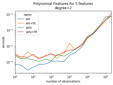
../_images/faster_polynomial_features_14_0.png

The gain is mostly visible for small dimensions.

Comparison with 1000 observations #

In this experiment, the number of observations is fixed to 1000 but the number of features varies.

poly = PolynomialFeatures(degree=2)
ext = ExtendedFeatures(poly_degree=2)
# implementation of PolynomialFeatures in 0.20.2
extslow = ExtendedFeatures(poly_degree=2, kind="poly-slow")


res = []
for n in [1, 2, 3, 4, 5, 6, 7, 8, 9, 10, 15, 20, 40, 50]:
    X = numpy.random.random((1000, n))
    poly.fit(X)
    ext.fit(X)
    extslow.fit(X)
    r1 = measure_time("poly.transform(X)", context=dict(X=X, poly=poly), repeat=5, number=30, div_by_number=True)
    r2 = measure_time("ext.transform(X)", context=dict(X=X, ext=ext), repeat=5, number=30, div_by_number=True)
    r3 = measure_time("extslow.transform(X)", context=dict(X=X, extslow=extslow), repeat=5, number=30, div_by_number=True)
    r1["name"] = "poly"
    r2["name"] = "ext"
    r3["name"] = "extslow"
    r1["nfeat"] = n
    r2["nfeat"] = n
    r3["nfeat"] = n
    x1 = poly.transform(X)
    x2 = ext.transform(X)
    x3 = extslow.transform(X)
    r1["numf"] = x1.shape[1]
    r2["numf"] = x2.shape[1]
    r3["numf"] = x3.shape[1]
    res.append(r1)
    res.append(r2)
    res.append(r3)

import pandas
df = pandas.DataFrame(res)
df.tail()

	average	deviation	min_exec	max_exec	repeat	number	context_size	name	nfeat	numf
37	0.009331	0.001603	0.008280	0.012519	5	30	240	ext	40	861
38	0.022619	0.002868	0.018793	0.026324	5	30	240	extslow	40	861
39	0.013188	0.000370	0.012828	0.013888	5	30	240	poly	50	1326
40	0.012817	0.000102	0.012700	0.012951	5	30	240	ext	50	1326
41	0.030384	0.000717	0.029955	0.031813	5	30	240	extslow	50	1326

piv = df.pivot("nfeat", "name", "average")
piv[:5]

name	ext	extslow	poly
nfeat
1	0.000026	0.000059	0.000152
2	0.000055	0.000100	0.000113
3	0.000161	0.000381	0.000237
4	0.000148	0.000221	0.000219
5	0.000185	0.000340	0.000236

ax = piv.plot(logy=True, logx=True)
ax.set_title("Polynomial Features for 1000 observations\ndegree=2")
ax.set_ylabel("seconds")
ax.set_xlabel("number of features");

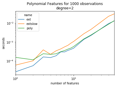
../_images/faster_polynomial_features_19_0.png

It is twice faster.

Comparison for different degrees #

In this experiment, the number of observations and features is fixed, the degree increases.

res = []
for n in [2, 3, 4, 5, 6, 7, 8]:
    X = numpy.random.random((1000, 4))
    poly = PolynomialFeatures(degree=n)
    ext = ExtendedFeatures(poly_degree=n)
    poly.fit(X)
    ext.fit(X)
    r1 = measure_time("poly.transform(X)", context=dict(X=X, poly=poly), repeat=5, number=30, div_by_number=True)
    r2 = measure_time("ext.transform(X)", context=dict(X=X, ext=ext), repeat=5, number=30, div_by_number=True)
    r1["name"] = "poly"
    r2["name"] = "ext"
    r1["degree"] = n
    r2["degree"] = n
    x1 = poly.transform(X)
    x2 = ext.transform(X)
    r1["numf"] = x1.shape[1]
    r2["numf"] = x2.shape[1]
    res.append(r1)
    res.append(r2)

import pandas
df = pandas.DataFrame(res)
df.tail()

	average	deviation	min_exec	max_exec	repeat	number	context_size	name	degree	numf
9	0.001960	0.000067	0.001915	0.002094	5	30	240	ext	6	210
10	0.003131	0.000118	0.003009	0.003327	5	30	240	poly	7	330
11	0.003076	0.000233	0.002845	0.003393	5	30	240	ext	7	330
12	0.004299	0.000046	0.004243	0.004367	5	30	240	poly	8	495
13	0.004157	0.000035	0.004114	0.004217	5	30	240	ext	8	495

piv = df.pivot("degree", "name", "average")
piv[:5]

name	ext	poly
degree
2	0.000140	0.000312
3	0.000304	0.000363
4	0.000506	0.000579
5	0.000715	0.000789
6	0.001960	0.002032

ax = piv.plot(logy=True, logx=True)
ax.set_title("Polynomial Features for 1000 observations\nnumber of features is 4")
ax.set_ylabel("seconds")
ax.set_xlabel("degree");

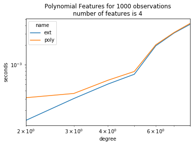
../_images/faster_polynomial_features_24_0.png

It is worth transposing.

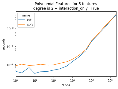
Same experiment with interaction_only=True #

res = []
for n in [1, 2, 5, 10, 20, 50, 100, 200, 500, 1000, 2000,
          5000, 10000, 20000, 50000, 100000, 200000]:
    poly = PolynomialFeatures(degree=2, interaction_only=True)
    ext = ExtendedFeatures(poly_degree=2, poly_interaction_only=True)
    X = numpy.random.random((n, 5))
    poly.fit(X)
    ext.fit(X)
    r1 = measure_time("poly.transform(X)", context=dict(X=X, poly=poly), repeat=2, number=30, div_by_number=True)
    r2 = measure_time("ext.transform(X)", context=dict(X=X, ext=ext), repeat=2, number=30, div_by_number=True)
    r1["name"] = "poly"
    r2["name"] = "ext"
    r1["size"] = n
    r2["size"] = n
    res.append(r1)
    res.append(r2)

import pandas
df = pandas.DataFrame(res)
df.tail()

	average	deviation	min_exec	max_exec	repeat	number	context_size	name	size
29	0.010691	0.000073	0.010618	0.010764	2	30	240	ext	50000
30	0.026612	0.000794	0.025817	0.027406	2	30	240	poly	100000
31	0.025052	0.001583	0.023469	0.026635	2	30	240	ext	100000
32	0.058772	0.001345	0.057427	0.060118	2	30	240	poly	200000
33	0.054771	0.004555	0.050216	0.059327	2	30	240	ext	200000

piv = df.pivot("size", "name", "average")
piv[:5]

name	ext	poly
size
1	0.000042	0.000086
2	0.000034	0.000104
5	0.000068	0.000089
10	0.000032	0.000092
20	0.000040	0.000103

ax = piv.plot(logy=True, logx=True)
ax.set_title("Polynomial Features for 5 features\ndegree is 2 + interaction_only=True")
ax.set_ylabel("seconds")
ax.set_xlabel("N obs");

../_images/faster_polynomial_features_29_0.png

Memory profiler #

from memory_profiler import memory_usage
poly = PolynomialFeatures(degree=2, interaction_only=True)
poly.fit(X)
memory_usage((poly.transform, (X,)), interval=0.1, max_usage=True)

258.02734375

def pick_value(v):
    try:
        return v[0]
    except TypeError:
        return v

res = []
for n in [10000, 50000, 100000, 200000]:
    X = numpy.random.random((n, 50))
    print(n)
    poly = PolynomialFeatures(degree=2, interaction_only=True)
    ext = ExtendedFeatures(poly_degree=2, poly_interaction_only=True)
    poly.fit(X)
    ext.fit(X)
    r1 = memory_usage((poly.transform, (X,)), interval=0.1, max_usage=True)
    r2 = memory_usage((ext.transform, (X,)), interval=0.1, max_usage=True)
    r1 = {"memory": pick_value(r1)}
    r2 = {"memory": pick_value(r2)}
    r1["name"] = "poly"
    r2["name"] = "ext"
    r1["size"] = n
    r2["size"] = n
    res.append(r1)
    res.append(r2)

import pandas
df = pandas.DataFrame(res)
df.tail()

	memory	name	size
3	699.679688	ext	50000
4	1243.664062	poly	100000
5	1205.515625	ext	100000
6	1952.316406	poly	200000
7	2029.765625	ext	200000

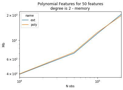
piv = df.pivot("size", "name", "memory")
piv[:5]

name	ext	poly
size
10000	392.445312	396.347656
50000	699.679688	718.839844
100000	1205.515625	1243.664062
200000	2029.765625	1952.316406

ax = piv.plot(logy=True, logx=True)
ax.set_title("Polynomial Features for 50 features\ndegree is 2 - memory")
ax.set_ylabel("Mb")
ax.set_xlabel("N obs");

../_images/faster_polynomial_features_34_0.png

Faster Polynomial Features#

Polynomial Features#

Comparison with 5 features#

Comparison with 1000 observations#

Comparison for different degrees#

Same experiment with interaction_only=True#

Memory profiler#