ONNX visualization#
Links: notebook, html, PDF, python, slides, GitHub
ONNX is a serialization format for machine learned model. It is a list of mathematical functions used to describe every prediction function for standard and deep machine learning. Module onnx offers some tools to display ONNX graph. Netron is another approach. The following notebooks explore a ligher visualization.
from jyquickhelper import add_notebook_menu
add_notebook_menu()
Train a model#
from sklearn.datasets import load_iris
from sklearn.model_selection import train_test_split
from sklearn.linear_model import LogisticRegression
iris = load_iris()
X, y = iris.data, iris.target
X_train, X_test, y_train, y_test = train_test_split(X, y)
clr = LogisticRegression(solver='liblinear')
clr.fit(X_train, y_train)
LogisticRegression(solver='liblinear')
Convert a model#
import numpy
from mlprodict.onnx_conv import to_onnx
model_onnx = to_onnx(clr, X_train.astype(numpy.float32))
Explore it with OnnxInference#
from mlprodict.onnxrt import OnnxInference

sess = OnnxInference(model_onnx)
sess
OnnxInference(...)
print(sess)
OnnxInference(...)
    ir_version: 4
    producer_name: "skl2onnx"
    producer_version: "1.7.1076"
    domain: "ai.onnx"
    model_version: 0
    doc_string: ""
    graph {
      node {
        input: "X"
        output: "label"
        output: "probability_tensor"
        name: "LinearClassifier"
        op_type: "LinearClassifier"
        attribute {
          name: "classlabels_ints"
          ints: 0
          ints: 1
          ints: 2
          type: INTS
        }
        attribute {
          name: "coefficients"
          floats: 0.3895888328552246
          floats: 1.3643852472305298
          floats: -2.140394449234009
          floats: -0.9475928544998169
          floats: 0.3562876284122467
          floats: -1.4181873798370361
          floats: 0.5958272218704224
          floats: -1.3317818641662598
          floats: -1.5090725421905518
          floats: -1.3937636613845825
          floats: 2.168299436569214
          floats: 2.3770956993103027
          type: FLOATS
        }
        attribute {
          name: "intercepts"
          floats: 0.23760676383972168
          floats: 0.8039277791976929
          floats: -1.0647538900375366
          type: FLOATS
        }
        attribute {
          name: "multi_class"
          i: 1
          type: INT
        }
        attribute {
          name: "post_transform"
          s: "LOGISTIC"
          type: STRING
        }
        domain: "ai.onnx.ml"
      }
      node {
        input: "probability_tensor"
        output: "probabilities"
        name: "Normalizer"
        op_type: "Normalizer"
        attribute {
          name: "norm"
          s: "L1"
          type: STRING
        }
        domain: "ai.onnx.ml"
      }
      node {
        input: "label"
        output: "output_label"
        name: "Cast"
        op_type: "Cast"
        attribute {
          name: "to"
          i: 7
          type: INT
        }
        domain: ""
      }
      node {
        input: "probabilities"
        output: "output_probability"
        name: "ZipMap"
        op_type: "ZipMap"
        attribute {
          name: "classlabels_int64s"
          ints: 0
          ints: 1
          ints: 2
          type: INTS
        }
        domain: "ai.onnx.ml"
      }
      name: "mlprodict_ONNX(LogisticRegression)"
      input {
        name: "X"
        type {
          tensor_type {
            elem_type: 1
            shape {
              dim {
              }
              dim {
                dim_value: 4
              }
            }
          }
        }
      }
      output {
        name: "output_label"
        type {
          tensor_type {
            elem_type: 7
            shape {
              dim {
              }
            }
          }
        }
      }
      output {
        name: "output_probability"
        type {
          sequence_type {
            elem_type {
              map_type {
                key_type: 7
                value_type {
                  tensor_type {
                    elem_type: 1
                  }
                }
              }
            }
          }
        }
      }
    }
    opset_import {
      domain: "ai.onnx.ml"
      version: 1
    }
    opset_import {
      domain: ""
      version: 9
    }
dot#
dot = sess.to_dot()
print(dot)
digraph{
  ranksep=0.25;
  nodesep=0.05;
  orientation=portrait;
  X [shape=box color=red label="Xnfloat((0, 4))" fontsize=10];
  output_label [shape=box color=green label="output_labelnint64((0,))" fontsize=10];
  output_probability [shape=box color=green label="output_probabilityn[{int64, {'kind': 'tensor', 'elem': 'float', 'shape': }}]" fontsize=10];

  label [shape=box label="label" fontsize=10];
  probability_tensor [shape=box label="probability_tensor" fontsize=10];
  LinearClassifier [shape=box style="filled,rounded" color=orange label="LinearClassifiern(LinearClassifier)nclasslabels_ints=[0 1 2]ncoefficients=[ 0.38958883  1.36...nintercepts=[ 0.23760676  0.8039...nmulti_class=1npost_transform=b'LOGISTIC'" fontsize=10];
  X -> LinearClassifier;
  LinearClassifier -> label;
  LinearClassifier -> probability_tensor;
  probabilities [shape=box label="probabilities" fontsize=10];
  Normalizer [shape=box style="filled,rounded" color=orange label="Normalizern(Normalizer)nnorm=b'L1'" fontsize=10];
  probability_tensor -> Normalizer;
  Normalizer -> probabilities;
  Cast [shape=box style="filled,rounded" color=orange label="Castn(Cast)nto=7" fontsize=10];
  label -> Cast;
  Cast -> output_label;
  ZipMap [shape=box style="filled,rounded" color=orange label="ZipMapn(ZipMap)nclasslabels_int64s=[0 1 2]" fontsize=10];
  probabilities -> ZipMap;
  ZipMap -> output_probability;
}
from jyquickhelper import RenderJsDot
RenderJsDot(dot)  # add local=True if nothing shows up
magic commands#
The module implements a magic command to easily display graphs.
%load_ext mlprodict
The mlprodict extension is already loaded. To reload it, use:
  %reload_ext mlprodict
# add -l 1 if nothing shows up
%onnxview model_onnx
Shape information#
It is possible to use the python runtime to get an estimation of each node shape.
%onnxview model_onnx -a 1
The shape (n, 2) means a matrix with an indefinite number of rows
and 2 columns.
runtime#
Let’s compute the prediction using a Python runtime.
prob = sess.run({'X': X_test})['output_probability']
prob[:5]
{0: array([0.84339281, 0.01372288, 0.77424892, 0.00095374, 0.04052374]),
 1: array([0.15649399, 0.71819778, 0.22563196, 0.25979154, 0.7736001 ]),
 2: array([1.13198419e-04, 2.68079336e-01, 1.19117272e-04, 7.39254721e-01,
        1.85876160e-01])}
import pandas
prob = pandas.DataFrame(list(prob)).values
prob[:5]
array([[8.43392810e-01, 1.56493992e-01, 1.13198419e-04],
       [1.37228844e-02, 7.18197780e-01, 2.68079336e-01],
       [7.74248918e-01, 2.25631964e-01, 1.19117272e-04],
       [9.53737402e-04, 2.59791542e-01, 7.39254721e-01],
       [4.05237433e-02, 7.73600097e-01, 1.85876160e-01]])
Which we compare to the original model.
clr.predict_proba(X_test)[:5]
array([[8.43392800e-01, 1.56494002e-01, 1.13198441e-04],
       [1.37228764e-02, 7.18197725e-01, 2.68079398e-01],
       [7.74248907e-01, 2.25631976e-01, 1.19117296e-04],
       [9.53736800e-04, 2.59791543e-01, 7.39254720e-01],
       [4.05237263e-02, 7.73600070e-01, 1.85876204e-01]])
Some time measurement…
%timeit clr.predict_proba(X_test)
86.7 µs ± 7.33 µs per loop (mean ± std. dev. of 7 runs, 10000 loops each)
%timeit sess.run({'X': X_test})['output_probability']
52.5 µs ± 4.53 µs per loop (mean ± std. dev. of 7 runs, 10000 loops each)
With one observation:
%timeit clr.predict_proba(X_test[:1])
77.6 µs ± 4.07 µs per loop (mean ± std. dev. of 7 runs, 10000 loops each)
%timeit sess.run({'X': X_test[:1]})['output_probability']
40.6 µs ± 913 ns per loop (mean ± std. dev. of 7 runs, 10000 loops each)
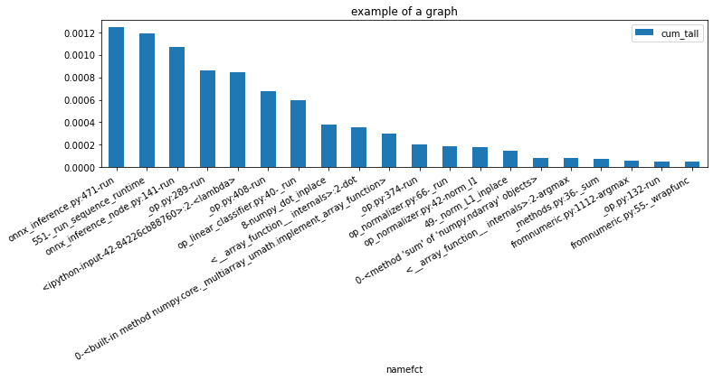
%matplotlib inline
from pyquickhelper.pycode.profiling import profile
pr, df = profile(lambda: sess.run({'X': X_test})['output_probability'], as_df=True)
ax = df[['namefct', 'cum_tall']].head(n=20).set_index('namefct').plot(kind='bar', figsize=(12, 3), rot=30)
ax.set_title("example of a graph")
for la in ax.get_xticklabels():
    la.set_horizontalalignment('right');
Add metadata#
It is possible to add metadata once the model is converted.
meta = model_onnx.metadata_props.add()
meta.key = "key_meta"
meta.value = "value_meta"
list(model_onnx.metadata_props)
[key: "key_meta"
 value: "value_meta"]
model_onnx.metadata_props[0]
key: "key_meta"
value: "value_meta"
Simple PCA#
from sklearn.decomposition import PCA
model = PCA(n_components=2)
model.fit(X)
PCA(n_components=2)
pca_onnx = to_onnx(model, X.astype(numpy.float32))
%load_ext mlprodict
The mlprodict extension is already loaded. To reload it, use:
  %reload_ext mlprodict
%onnxview pca_onnx -a 1
The graph would probably be faster if the multiplication was done before the subtraction because it is easier to do this one inline than the multiplication.