Train and deploy a scikit-learn pipeline

This program starts from an example in scikit-learn documentation: Plot individual and voting regression predictions, converts it into ONNX and finally computes the predictions a different runtime.

Training a pipeline

from pyquickhelper.helpgen.graphviz_helper import plot_graphviz
import numpy
from onnxruntime import InferenceSession
from sklearn.datasets import load_diabetes
from sklearn.ensemble import (
    GradientBoostingRegressor, RandomForestRegressor,
    VotingRegressor)
from sklearn.linear_model import LinearRegression
from sklearn.model_selection import train_test_split
from sklearn.pipeline import Pipeline
from skl2onnx import to_onnx
from mlprodict.onnxrt import OnnxInference


X, y = load_diabetes(return_X_y=True)
X_train, X_test, y_train, y_test = train_test_split(X, y)

# Train classifiers
reg1 = GradientBoostingRegressor(random_state=1, n_estimators=5)
reg2 = RandomForestRegressor(random_state=1, n_estimators=5)
reg3 = LinearRegression()

ereg = Pipeline(steps=[
    ('voting', VotingRegressor([('gb', reg1), ('rf', reg2), ('lr', reg3)])),
])
ereg.fit(X_train, y_train)

Pipeline(steps=[('voting',
                 VotingRegressor(estimators=[('gb',
                                              GradientBoostingRegressor(n_estimators=5,
                                                                        random_state=1)),
                                             ('rf',
                                              RandomForestRegressor(n_estimators=5,
                                                                    random_state=1)),
                                             ('lr', LinearRegression())]))])

In a Jupyter environment, please rerun this cell to show the HTML representation or trust the notebook.
On GitHub, the HTML representation is unable to render, please try loading this page with nbviewer.org.

Converts the model

The second argument gives a sample of the data used to train the model. It is used to infer the input type of the ONNX graph. It is converted into single float and ONNX runtimes may not fully support doubles.

onx = to_onnx(ereg, X_train[:1].astype(numpy.float32),
              target_opset={'': 14, 'ai.onnx.ml': 2})

Prediction with ONNX

The first example uses onnxruntime.

sess = InferenceSession(onx.SerializeToString(),
                        providers=['CPUExecutionProvider'])
pred_ort = sess.run(None, {'X': X_test.astype(numpy.float32)})[0]

pred_skl = ereg.predict(X_test.astype(numpy.float32))

pred_ort[:5], pred_skl[:5]

(array([[178.8722  ],
       [152.20142 ],
       [135.78523 ],
       [108.934006],
       [107.454346]], dtype=float32), array([178.87218557, 152.20140568, 135.78523473, 108.93399505,
       107.45433764]))

Comparison

Before deploying, we need to compare that both scikit-learn and ONNX return the same predictions.

def diff(p1, p2):
    p1 = p1.ravel()
    p2 = p2.ravel()
    d = numpy.abs(p2 - p1)
    return d.max(), (d / numpy.abs(p1)).max()


print(diff(pred_skl, pred_ort))

(2.5759757733112565e-05, 1.2627913765785005e-07)

It looks good. Biggest errors (absolute and relative) are within the margin error introduced by using floats instead of doubles. We can save the model into ONNX format and compute the same predictions in many platform using onnxruntime.

Python runtime

A python runtime can be used as well to compute the prediction. It is not meant to be used into production (it still relies on python), but it is useful to investigate why the conversion went wrong. It uses module mlprodict.

oinf = OnnxInference(onx, runtime="python_compiled")
print(oinf)

OnnxInference(...)
    def compiled_run(dict_inputs, yield_ops=None, context=None, attributes=None):
        if yield_ops is not None:
            raise NotImplementedError('yields_ops should be None.')
        # init: w0 (w0)
        # inputs
        X = dict_inputs['X']
        (var_1, ) = n0_treeensembleregressor_1(X)
        (var_0, ) = n1_treeensembleregressor_1(X)
        (var_2, ) = n2_linearregressor(X)
        (wvar_0, ) = n3_mul(var_0, w0)
        (wvar_1, ) = n4_mul(var_1, w0)
        (wvar_2, ) = n5_mul(var_2, w0)
        (fvar_0, ) = n6_flatten(wvar_0)
        (fvar_2, ) = n7_flatten(wvar_2)
        (fvar_1, ) = n8_flatten(wvar_1)
        (variable, ) = n9_sum(fvar_0, fvar_1, fvar_2)
        return {
            'variable': variable,
        }

It works almost the same way.

pred_pyrt = oinf.run({'X': X_test.astype(numpy.float32)})['variable']
print(diff(pred_skl, pred_pyrt))

(2.5759757733112565e-05, 1.7072610407737767e-07)

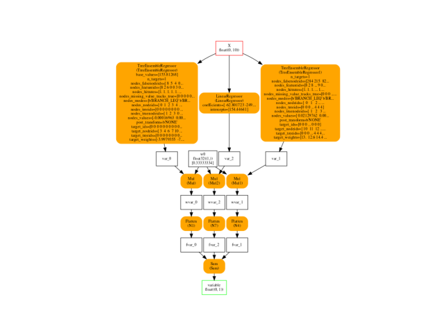
Final graph

ax = plot_graphviz(oinf.to_dot(), dpi=100)
ax.get_xaxis().set_visible(False)
ax.get_yaxis().set_visible(False)