Benchmark ONNX conversion

Example Train and deploy a scikit-learn pipeline converts a simple model. This example takes a similar example but on random data and compares the processing time required by each option to compute predictions.

Training a pipeline

import numpy
from pandas import DataFrame
from tqdm import tqdm
from sklearn import config_context
from sklearn.datasets import make_regression
from sklearn.ensemble import (
    GradientBoostingRegressor, RandomForestRegressor,
    VotingRegressor)
from sklearn.linear_model import LinearRegression
from sklearn.model_selection import train_test_split
from mlprodict.onnxrt import OnnxInference
from onnxruntime import InferenceSession
from skl2onnx import to_onnx
from onnxcustom.utils import measure_time


N = 11000
X, y = make_regression(N, n_features=10)
X_train, X_test, y_train, y_test = train_test_split(
    X, y, train_size=0.01)
print("Train shape", X_train.shape)
print("Test shape", X_test.shape)

reg1 = GradientBoostingRegressor(random_state=1)
reg2 = RandomForestRegressor(random_state=1)
reg3 = LinearRegression()
ereg = VotingRegressor([('gb', reg1), ('rf', reg2), ('lr', reg3)])
ereg.fit(X_train, y_train)

Train shape (110, 10)
Test shape (10890, 10)

VotingRegressor(estimators=[('gb', GradientBoostingRegressor(random_state=1)),
                            ('rf', RandomForestRegressor(random_state=1)),
                            ('lr', LinearRegression())])

In a Jupyter environment, please rerun this cell to show the HTML representation or trust the notebook.
On GitHub, the HTML representation is unable to render, please try loading this page with nbviewer.org.

Measure the processing time

We use function measure_time. The page about assume_finite may be useful if you need to optimize the prediction. We measure the processing time per observation whether or not an observation belongs to a batch or is a single one.

sizes = [(1, 50), (10, 50), (1000, 10), (10000, 5)]

with config_context(assume_finite=True):
    obs = []
    for batch_size, repeat in tqdm(sizes):
        context = {"ereg": ereg, 'X': X_test[:batch_size]}
        mt = measure_time(
            "ereg.predict(X)", context, div_by_number=True,
            number=10, repeat=repeat)
        mt['size'] = context['X'].shape[0]
        mt['mean_obs'] = mt['average'] / mt['size']
        obs.append(mt)

df_skl = DataFrame(obs)
df_skl

  0%|          | 0/4 [00:00<?, ?it/s]
 25%|##5       | 1/4 [00:15<00:45, 15.00s/it]
 50%|#####     | 2/4 [00:29<00:29, 14.83s/it]
 75%|#######5  | 3/4 [00:34<00:10, 10.20s/it]
100%|##########| 4/4 [00:42<00:00,  9.37s/it]
100%|##########| 4/4 [00:42<00:00, 10.63s/it]

	average	deviation	min_exec	max_exec	repeat	number	size	mean_obs
0	0.029989	0.000107	0.029839	0.030542	50	10	1	0.029989
1	0.029418	0.000125	0.029245	0.030009	50	10	10	0.002942
2	0.046801	0.003460	0.043296	0.053204	10	10	1000	0.000047
3	0.162123	0.000081	0.162050	0.162258	5	10	10000	0.000016

Graphe.

df_skl.set_index('size')[['mean_obs']].plot(
    title="scikit-learn", logx=True, logy=True)

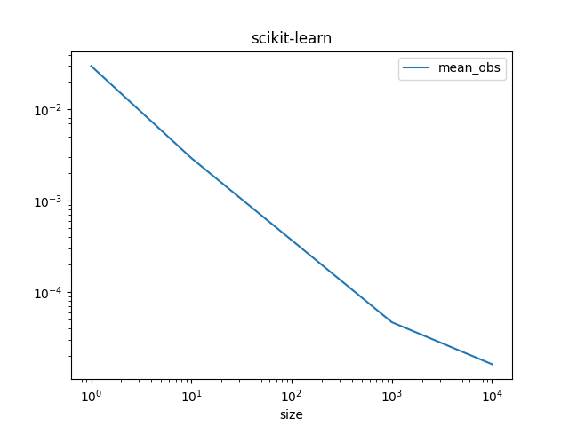
<AxesSubplot: title={'center': 'scikit-learn'}, xlabel='size'>

ONNX runtime

The same is done with the two ONNX runtime available.

onx = to_onnx(ereg, X_train[:1].astype(numpy.float32),
              target_opset={'': 14, 'ai.onnx.ml': 2})
sess = InferenceSession(onx.SerializeToString(),
                        providers=['CPUExecutionProvider'])
oinf = OnnxInference(onx, runtime="python_compiled")

obs = []
for batch_size, repeat in tqdm(sizes):

    # scikit-learn
    context = {"ereg": ereg, 'X': X_test[:batch_size].astype(numpy.float32)}
    mt = measure_time(
        "ereg.predict(X)", context, div_by_number=True,
        number=10, repeat=repeat)
    mt['size'] = context['X'].shape[0]
    mt['skl'] = mt['average'] / mt['size']

    # onnxruntime
    context = {"sess": sess, 'X': X_test[:batch_size].astype(numpy.float32)}
    mt2 = measure_time(
        "sess.run(None, {'X': X})[0]", context, div_by_number=True,
        number=10, repeat=repeat)
    mt['ort'] = mt2['average'] / mt['size']

    # mlprodict
    context = {"oinf": oinf, 'X': X_test[:batch_size].astype(numpy.float32)}
    mt2 = measure_time(
        "oinf.run({'X': X})['variable']", context, div_by_number=True,
        number=10, repeat=repeat)
    mt['pyrt'] = mt2['average'] / mt['size']

    # end
    obs.append(mt)


df = DataFrame(obs)
df

  0%|          | 0/4 [00:00<?, ?it/s]
 25%|##5       | 1/4 [00:20<01:00, 20.20s/it]
 50%|#####     | 2/4 [00:42<00:43, 21.63s/it]
 75%|#######5  | 3/4 [01:12<00:25, 25.23s/it]
100%|##########| 4/4 [02:34<00:00, 47.79s/it]
100%|##########| 4/4 [02:34<00:00, 38.68s/it]

	average	deviation	min_exec	max_exec	repeat	number	size	skl	ort	pyrt
0	0.030600	0.000161	0.030286	0.031162	50	10	1	0.030600	0.000234	0.009540
1	0.030283	0.000084	0.030121	0.030600	50	10	10	0.003028	0.000057	0.001440
2	0.045175	0.001052	0.044146	0.047618	10	10	1000	0.000045	0.000006	0.000244
3	0.164668	0.000791	0.163987	0.166081	5	10	10000	0.000016	0.000003	0.000145

Graph.

df.set_index('size')[['skl', 'ort', 'pyrt']].plot(
    title="Average prediction time per runtime",
    logx=True, logy=True)

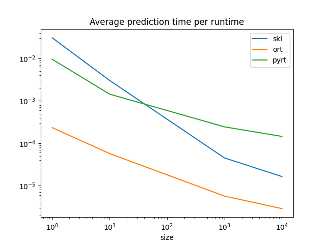
<AxesSubplot: title={'center': 'Average prediction time per runtime'}, xlabel='size'>

ONNX runtimes are much faster than scikit-learn to predict one observation. scikit-learn is optimized for training, for batch prediction. That explains why scikit-learn and ONNX runtimes seem to converge for big batches. They use similar implementation, parallelization and languages (C++, openmp).