Funny discrepancies

Function sigmoid is . For small or high value, implementation has to do approximation and they are not always the same. It may be a tradeoff between precision and computation time… It is always a tradeoff.

Precision

This section compares the precision of a couple of implementations of the ssigmoid function. The custom implementation is done with a Taylor expansion of exponential function: .

import time
import numpy
import pandas
from tqdm import tqdm
from scipy.special import expit

from skl2onnx.algebra.onnx_ops import OnnxSigmoid
from skl2onnx.common.data_types import FloatTensorType
from onnxruntime import InferenceSession
from mlprodict.onnxrt import OnnxInference
from onnxcustom import get_max_opset
import matplotlib.pyplot as plt

one = numpy.array([1], dtype=numpy.float64)


def taylor_approximation_exp(x, degre=50):
    y = numpy.zeros(x.shape, dtype=x.dtype)
    a = numpy.ones(x.shape, dtype=x.dtype)
    for i in range(1, degre + 1):
        a *= x / i
        y += a
    return y


def taylor_sigmoid(x, degre=50):
    den = one + taylor_approximation_exp(-x, degre)
    return one / (den)


opset = get_max_opset()
N = 300
min_values = [-20 + float(i) * 10 / N for i in range(N)]
data = numpy.array([0], dtype=numpy.float32)

node = OnnxSigmoid('X', op_version=opset, output_names=['Y'])
onx = node.to_onnx({'X': FloatTensorType()},
                   {'Y': FloatTensorType()},
                   target_opset=opset)
rts = ['numpy', 'python', 'onnxruntime', 'taylor20', 'taylor40']

oinf = OnnxInference(onx)
sess = InferenceSession(onx.SerializeToString())

graph = []
for mv in tqdm(min_values):
    data[0] = mv
    for rt in rts:
        lab = ""
        if rt == 'numpy':
            y = expit(data)
        elif rt == 'python':
            y = oinf.run({'X': data})['Y']
            # * 1.2 to avoid curves to be superimposed
            y *= 1.2
            lab = "x1.2"
        elif rt == 'onnxruntime':
            y = sess.run(None, {'X': data})[0]
        elif rt == 'taylor40':
            y = taylor_sigmoid(data, 40)
            # * 0.8 to avoid curves to be superimposed
            y *= 0.8
            lab = "x0.8"
        elif rt == 'taylor20':
            y = taylor_sigmoid(data, 20)
            # * 0.6 to avoid curves to be superimposed
            y *= 0.6
            lab = "x0.6"
        else:
            raise AssertionError(f"Unknown runtime {rt!r}.")
        value = y[0]
        graph.append(dict(rt=rt + lab, x=mv, y=value))

  0%|          | 0/300 [00:00<?, ?it/s]
 11%|#1        | 34/300 [00:00<00:00, 335.98it/s]
 26%|##6       | 78/300 [00:00<00:00, 392.91it/s]
 41%|####      | 122/300 [00:00<00:00, 411.56it/s]
 55%|#####5    | 166/300 [00:00<00:00, 420.21it/s]
 70%|#######   | 210/300 [00:00<00:00, 425.67it/s]
 85%|########4 | 254/300 [00:00<00:00, 428.45it/s]
 99%|#########9| 298/300 [00:00<00:00, 430.18it/s]
100%|##########| 300/300 [00:00<00:00, 419.26it/s]

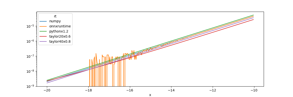
Graph.

_, ax = plt.subplots(1, 1, figsize=(12, 4))
df = pandas.DataFrame(graph)
piv = df.pivot('x', 'rt', 'y')
print(piv.T.head())
piv.plot(ax=ax, logy=True)

x               -20.000000    -19.966667  ...  -10.066667  -10.033333
rt                                        ...
numpy         2.061154e-09  2.131016e-09  ...    0.000042    0.000044
onnxruntime  -5.960464e-08 -5.960464e-08  ...    0.000042    0.000044
pythonx1.2    2.473385e-09  2.557219e-09  ...    0.000051    0.000053
taylor20x0.6  2.211963e-09  2.274888e-09  ...    0.000026    0.000026
taylor40x0.8  1.648965e-09  1.704854e-09  ...    0.000034    0.000035

[5 rows x 300 columns]

<AxesSubplot: xlabel='x'>

. When x is very negative, . That explains the graph. We also see onnxruntime is less precise for these values. What’s the benefit?

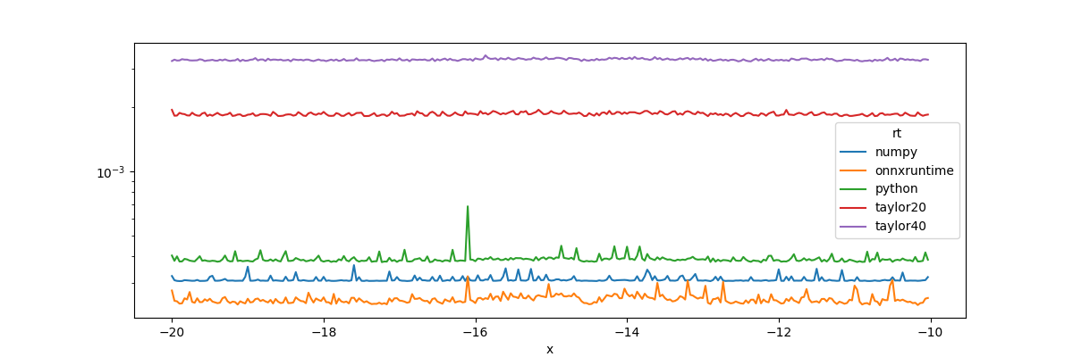
Computation time

graph = []
for mv in tqdm(min_values):
    data = numpy.array([mv] * 10000, dtype=numpy.float32)
    for rt in rts:
        begin = time.perf_counter()
        if rt == 'numpy':
            y = expit(data)
        elif rt == 'python':
            y = oinf.run({'X': data})['Y']
        elif rt == 'onnxruntime':
            y = sess.run(None, {'X': data})[0]
        elif rt == 'taylor40':
            y = taylor_sigmoid(data, 40)
        elif rt == 'taylor20':
            y = taylor_sigmoid(data, 20)
        else:
            raise AssertionError(f"Unknown runtime {rt!r}.")
        duration = time.perf_counter() - begin
        graph.append(dict(rt=rt, x=mv, y=duration))

_, ax = plt.subplots(1, 1, figsize=(12, 4))
df = pandas.DataFrame(graph)
piv = df.pivot('x', 'rt', 'y')
piv.plot(ax=ax, logy=True)

  0%|          | 0/300 [00:00<?, ?it/s]
  5%|5         | 15/300 [00:00<00:02, 140.70it/s]
 10%|#         | 30/300 [00:00<00:01, 140.32it/s]
 15%|#5        | 45/300 [00:00<00:01, 140.00it/s]
 20%|##        | 60/300 [00:00<00:01, 139.85it/s]
 25%|##4       | 74/300 [00:00<00:01, 139.79it/s]
 30%|##9       | 89/300 [00:00<00:01, 139.90it/s]
 34%|###4      | 103/300 [00:00<00:01, 139.79it/s]
 39%|###9      | 117/300 [00:00<00:01, 139.64it/s]
 44%|####3     | 131/300 [00:00<00:01, 139.03it/s]
 48%|####8     | 145/300 [00:01<00:01, 138.64it/s]
 53%|#####3    | 159/300 [00:01<00:01, 138.18it/s]
 58%|#####7    | 173/300 [00:01<00:00, 138.50it/s]
 62%|######2   | 187/300 [00:01<00:00, 138.09it/s]
 67%|######7   | 201/300 [00:01<00:00, 138.02it/s]
 72%|#######1  | 215/300 [00:01<00:00, 138.10it/s]
 76%|#######6  | 229/300 [00:01<00:00, 138.64it/s]
 81%|########1 | 243/300 [00:01<00:00, 138.94it/s]
 86%|########5 | 257/300 [00:01<00:00, 138.90it/s]
 90%|######### | 271/300 [00:01<00:00, 139.12it/s]
 95%|#########5| 285/300 [00:02<00:00, 139.35it/s]
100%|#########9| 299/300 [00:02<00:00, 139.37it/s]
100%|##########| 300/300 [00:02<00:00, 139.04it/s]

<AxesSubplot: xlabel='x'>

Conclusion

The implementation from onnxruntime is faster but is much less contiguous for extremes. It explains why probabilities may be much different when an observation is far from every classification border. In that case, onnxruntime implementation of the sigmoid function returns 0 when numpy.sigmoid() returns a smoother value. Probabilites of logistic regression are obtained after the raw scores are transformed with the sigmoid function and normalized. If the raw scores are very negative, the sum of probabilities becomes null with onnxruntime. The normalization fails.

# plt.show()