Transfer Learning with ONNX

Transfer learning is common with deep learning. A deep learning model is used as preprocessing before the output is sent to a final classifier or regressor. It is not quite easy in this case to mix framework, scikit-learn with pytorch (or skorch), the Keras API for Tensorflow, tf.keras.wrappers.scikit_learn. Every combination requires work. ONNX reduces the number of platforms to support. Once the model is converted into ONNX, it can be inserted in any scikit-learn pipeline.

Retrieve and load a model

We download one model from the ONNX Zoo but the model could be trained and produced by another converter library.

from io import BytesIO
import onnx
from mlprodict.sklapi import OnnxTransformer
from sklearn.decomposition import PCA
from sklearn.pipeline import Pipeline
from mlinsights.plotting.gallery import plot_gallery_images
import matplotlib.pyplot as plt
from onnxcustom.utils.imagenet_classes import class_names
import numpy
from PIL import Image
from onnxruntime import InferenceSession
import os
import urllib.request


def download_file(url, name, min_size):
    if not os.path.exists(name):
        print(f"download '{url}'")
        with urllib.request.urlopen(url) as u:
            content = u.read()
        if len(content) < min_size:
            raise RuntimeError(
                f"Unable to download '{url}' due to\n{content}")
        print(f"downloaded {len(content)} bytes.")
        with open(name, "wb") as f:
            f.write(content)
    else:
        print(f"'{name}' already downloaded")


model_name = "squeezenet1.1-7.onnx"
url_name = ("https://github.com/onnx/models/raw/main/vision/"
            "classification/squeezenet/model")
url_name += "/" + model_name
download_file(url_name, model_name, 100000)

download 'https://github.com/onnx/models/raw/main/vision/classification/squeezenet/model/squeezenet1.1-7.onnx'
downloaded 4956208 bytes.

Loading the ONNX file and use it on one image.

sess = InferenceSession(model_name,
                        providers=['CPUExecutionProvider'])

for inp in sess.get_inputs():
    print(inp)

NodeArg(name='data', type='tensor(float)', shape=[1, 3, 224, 224])

The model expects a series of images of size [3, 224, 224].

Classifying an image

url = ("https://upload.wikimedia.org/wikipedia/commons/d/d2/"
       "East_Coker_elm%2C_2.jpg")
img = "East_Coker_elm.jpg"
download_file(url, img, 100000)

im0 = Image.open(img)
im = im0.resize((224, 224))
# im.show()

download 'https://upload.wikimedia.org/wikipedia/commons/d/d2/East_Coker_elm%2C_2.jpg'
downloaded 712230 bytes.

Image to numpy and predection.

def im2array(im):
    X = numpy.asarray(im)
    X = X.transpose(2, 0, 1)
    X = X.reshape(1, 3, 224, 224)
    return X


X = im2array(im)
out = sess.run(None, {'data': X.astype(numpy.float32)})
out = out[0]

print(out[0, :5])

[145.59464   55.067673  60.599747  46.29393   37.98244 ]

Interpretation

res = list(sorted((r, class_names[i]) for i, r in enumerate(out[0])))
print(res[-5:])

[(205.84172, 'Samoyed, Samoyede'), (212.0366, 'park bench'), (225.50684, 'lakeside, lakeshore'), (232.90251, 'fountain'), (258.10968, 'geyser')]

Classifying more images

The initial image is rotated, the answer is changing.

angles = [a * 2. for a in range(-6, 6)]
imgs = [(angle, im0.rotate(angle).resize((224, 224)))
        for angle in angles]


def classify(imgs):
    labels = []
    for angle, img in imgs:
        X = im2array(img)
        probs = sess.run(None, {'data': X.astype(numpy.float32)})[0]
        pl = list(sorted(
            ((r, class_names[i]) for i, r in enumerate(probs[0])),
            reverse=True))
        labels.append((angle, pl))
    return labels


climgs = classify(imgs)
for angle, res in climgs:
    print(f"angle={angle} - {res[:5]}")


plot_gallery_images([img[1] for img in imgs],
                    [img[1][0][1][:15] for img in climgs])

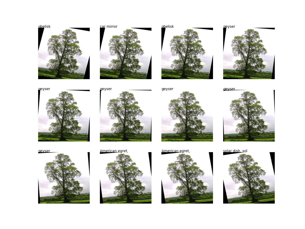
angle=-12.0 - [(247.06139, 'obelisk'), (238.95375, 'car mirror'), (235.27644, 'flagpole, flagstaff'), (231.51715, 'window screen'), (230.90665, 'picket fence, paling')]
angle=-10.0 - [(254.24683, 'car mirror'), (251.51355, 'obelisk'), (235.1051, 'groom, bridegroom'), (234.5295, 'picket fence, paling'), (232.13913, 'church, church building')]
angle=-8.0 - [(235.56947, 'obelisk'), (226.59702, 'car mirror'), (226.46767, 'picket fence, paling'), (221.46799, 'groom, bridegroom'), (220.8851, 'fountain')]
angle=-6.0 - [(265.50803, 'geyser'), (243.6862, 'obelisk'), (238.92964, 'fountain'), (226.73685, 'pedestal, plinth, footstall'), (226.11945, 'Great Pyrenees')]
angle=-4.0 - [(287.74472, 'geyser'), (255.25311, 'fountain'), (236.8495, 'obelisk'), (223.02892, 'Great Pyrenees'), (222.80464, 'church, church building')]
angle=-2.0 - [(267.63535, 'geyser'), (251.4896, 'fountain'), (214.64238, 'obelisk'), (214.56233, 'mobile home, manufactured home'), (213.12416, 'flagpole, flagstaff')]
angle=0.0 - [(258.10968, 'geyser'), (232.90251, 'fountain'), (225.50684, 'lakeside, lakeshore'), (212.0366, 'park bench'), (205.84172, 'Samoyed, Samoyede')]
angle=2.0 - [(222.7483, 'geyser'), (213.38457, 'fountain'), (212.24373, 'obelisk'), (198.37137, 'beacon, lighthouse, beacon light, pharos'), (197.43808, 'picket fence, paling')]
angle=4.0 - [(221.34749, 'geyser'), (209.60358, 'fountain'), (207.06915, 'American egret, great white heron, Egretta albus'), (201.63094, 'obelisk'), (198.75664, 'Great Pyrenees')]
angle=6.0 - [(230.98729, 'American egret, great white heron, Egretta albus'), (216.63416, 'fountain'), (212.7324, 'groom, bridegroom'), (209.60928, 'flagpole, flagstaff'), (209.46211, 'swimming trunks, bathing trunks')]
angle=8.0 - [(253.32701, 'American egret, great white heron, Egretta albus'), (222.69963, 'golf ball'), (222.50493, 'groom, bridegroom'), (222.36345, 'sulphur-crested cockatoo, Kakatoe galerita, Cacatua galerita'), (217.73135, 'swimming trunks, bathing trunks')]
angle=10.0 - [(244.30115, 'solar dish, solar collector, solar furnace'), (239.57332, 'flagpole, flagstaff'), (234.92137, 'picket fence, paling'), (230.62117, 'car mirror'), (221.87946, 'screen, CRT screen')]

array([[<AxesSubplot: >, <AxesSubplot: >, <AxesSubplot: >,
        <AxesSubplot: >],
       [<AxesSubplot: >, <AxesSubplot: >, <AxesSubplot: >,
        <AxesSubplot: >],
       [<AxesSubplot: >, <AxesSubplot: >, <AxesSubplot: >,
        <AxesSubplot: >]], dtype=object)

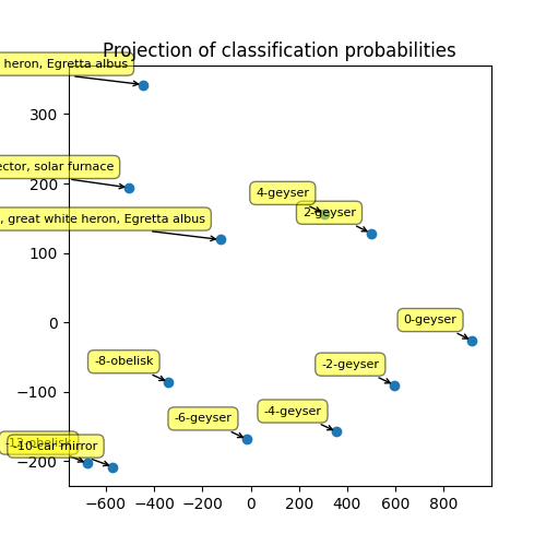
Transfer learning in a pipeline

The proposed transfer learning consists using a PCA to projet the probabilities on a graph.

with open(model_name, 'rb') as f:
    model_bytes = f.read()

pipe = Pipeline(steps=[
    ('deep', OnnxTransformer(
        model_bytes, runtime='onnxruntime1', change_batch_size=0)),
    ('pca', PCA(2))
])

X_train = numpy.vstack(
    [im2array(img) for _, img in imgs]).astype(numpy.float32)
pipe.fit(X_train)

proj = pipe.transform(X_train)
print(proj)

[[-676.576    -203.3546  ]
 [-570.6658   -208.0971  ]
 [-339.812     -86.339836]
 [ -14.555845 -168.44824 ]
 [ 357.2238   -157.61359 ]
 [ 596.38586   -90.210915]
 [ 918.8612    -26.340052]
 [ 499.87143   128.27255 ]
 [ 306.68604   156.42969 ]
 [-125.91182   119.21932 ]
 [-446.60452   342.45837 ]
 [-504.90277   194.02434 ]]

Graph for the PCA

fig, ax = plt.subplots(1, 1, figsize=(5, 5))
ax.plot(proj[:, 0], proj[:, 1], 'o')
ax.set_title("Projection of classification probabilities")
text = [f"{el[0]:1.0f}-{el[1][0][1]}" for el in climgs]
for label, x, y in zip(text, proj[:, 0], proj[:, 1]):
    ax.annotate(
        label, xy=(x, y), xytext=(-10, 10), fontsize=8,
        textcoords='offset points', ha='right', va='bottom',
        bbox=dict(boxstyle='round,pad=0.5', fc='yellow', alpha=0.5),
        arrowprops=dict(arrowstyle='->', connectionstyle='arc3,rad=0'))

Remove one layer at the end

The last is often removed before the model is inserted in a pipeline. Let’s see how to do that. First, we need the list of output for every node.

model_onnx = onnx.load(BytesIO(model_bytes))
outputs = []
for node in model_onnx.graph.node:
    print(node.name, node.output)
    outputs.extend(node.output)

squeezenet0_conv0_fwd ['squeezenet0_conv0_fwd']
squeezenet0_relu0_fwd ['squeezenet0_relu0_fwd']
squeezenet0_pool0_fwd ['squeezenet0_pool0_fwd']
squeezenet0_conv1_fwd ['squeezenet0_conv1_fwd']
squeezenet0_relu1_fwd ['squeezenet0_relu1_fwd']
squeezenet0_conv2_fwd ['squeezenet0_conv2_fwd']
squeezenet0_relu2_fwd ['squeezenet0_relu2_fwd']
squeezenet0_conv3_fwd ['squeezenet0_conv3_fwd']
squeezenet0_relu3_fwd ['squeezenet0_relu3_fwd']
squeezenet0_concat0 ['squeezenet0_concat0']
squeezenet0_conv4_fwd ['squeezenet0_conv4_fwd']
squeezenet0_relu4_fwd ['squeezenet0_relu4_fwd']
squeezenet0_conv5_fwd ['squeezenet0_conv5_fwd']
squeezenet0_relu5_fwd ['squeezenet0_relu5_fwd']
squeezenet0_conv6_fwd ['squeezenet0_conv6_fwd']
squeezenet0_relu6_fwd ['squeezenet0_relu6_fwd']
squeezenet0_concat1 ['squeezenet0_concat1']
squeezenet0_pool1_fwd ['squeezenet0_pool1_fwd']
squeezenet0_conv7_fwd ['squeezenet0_conv7_fwd']
squeezenet0_relu7_fwd ['squeezenet0_relu7_fwd']
squeezenet0_conv8_fwd ['squeezenet0_conv8_fwd']
squeezenet0_relu8_fwd ['squeezenet0_relu8_fwd']
squeezenet0_conv9_fwd ['squeezenet0_conv9_fwd']
squeezenet0_relu9_fwd ['squeezenet0_relu9_fwd']
squeezenet0_concat2 ['squeezenet0_concat2']
squeezenet0_conv10_fwd ['squeezenet0_conv10_fwd']
squeezenet0_relu10_fwd ['squeezenet0_relu10_fwd']
squeezenet0_conv11_fwd ['squeezenet0_conv11_fwd']
squeezenet0_relu11_fwd ['squeezenet0_relu11_fwd']
squeezenet0_conv12_fwd ['squeezenet0_conv12_fwd']
squeezenet0_relu12_fwd ['squeezenet0_relu12_fwd']
squeezenet0_concat3 ['squeezenet0_concat3']
squeezenet0_pool2_fwd ['squeezenet0_pool2_fwd']
squeezenet0_conv13_fwd ['squeezenet0_conv13_fwd']
squeezenet0_relu13_fwd ['squeezenet0_relu13_fwd']
squeezenet0_conv14_fwd ['squeezenet0_conv14_fwd']
squeezenet0_relu14_fwd ['squeezenet0_relu14_fwd']
squeezenet0_conv15_fwd ['squeezenet0_conv15_fwd']
squeezenet0_relu15_fwd ['squeezenet0_relu15_fwd']
squeezenet0_concat4 ['squeezenet0_concat4']
squeezenet0_conv16_fwd ['squeezenet0_conv16_fwd']
squeezenet0_relu16_fwd ['squeezenet0_relu16_fwd']
squeezenet0_conv17_fwd ['squeezenet0_conv17_fwd']
squeezenet0_relu17_fwd ['squeezenet0_relu17_fwd']
squeezenet0_conv18_fwd ['squeezenet0_conv18_fwd']
squeezenet0_relu18_fwd ['squeezenet0_relu18_fwd']
squeezenet0_concat5 ['squeezenet0_concat5']
squeezenet0_conv19_fwd ['squeezenet0_conv19_fwd']
squeezenet0_relu19_fwd ['squeezenet0_relu19_fwd']
squeezenet0_conv20_fwd ['squeezenet0_conv20_fwd']
squeezenet0_relu20_fwd ['squeezenet0_relu20_fwd']
squeezenet0_conv21_fwd ['squeezenet0_conv21_fwd']
squeezenet0_relu21_fwd ['squeezenet0_relu21_fwd']
squeezenet0_concat6 ['squeezenet0_concat6']
squeezenet0_conv22_fwd ['squeezenet0_conv22_fwd']
squeezenet0_relu22_fwd ['squeezenet0_relu22_fwd']
squeezenet0_conv23_fwd ['squeezenet0_conv23_fwd']
squeezenet0_relu23_fwd ['squeezenet0_relu23_fwd']
squeezenet0_conv24_fwd ['squeezenet0_conv24_fwd']
squeezenet0_relu24_fwd ['squeezenet0_relu24_fwd']
squeezenet0_concat7 ['squeezenet0_concat7']
squeezenet0_dropout0_fwd ['squeezenet0_dropout0_fwd']
squeezenet0_conv25_fwd ['squeezenet0_conv25_fwd']
squeezenet0_relu25_fwd ['squeezenet0_relu25_fwd']
squeezenet0_pool3_fwd ['squeezenet0_pool3_fwd']
squeezenet0_flatten0_reshape0 ['squeezenet0_flatten0_reshape0']

We select one of the last one.

selected = outputs[-3]
print("selected", selected)

selected squeezenet0_relu25_fwd

And we tell OnnxTransformer to use that specific one and to flatten the output as the dimension is not a matrix.

pipe2 = Pipeline(steps=[
    ('deep', OnnxTransformer(
        model_bytes, runtime='onnxruntime1', change_batch_size=0,
        output_name=selected, reshape=True)),
    ('pca', PCA(2))
])

pipe2.fit(X_train)

Pipeline(steps=[('deep',
                 OnnxTransformer(change_batch_size=0, onnx_bytes=b'\x08\x03:\xa5\xc0\xae\x02\n\xca\x01\n\x04data\n\x18squeezenet0_conv0_weight\n\x16squeezenet0_conv0_bias\x12\x15squeezenet0_conv0_fwd\x1a\x15squeezenet0_conv0_fwd"\x04Conv*\x12\n\tdilations@\x01@\x01\xa0\x01\x07*\x0c\n\x05group\x18\x01\xa0\x01\x02*\x15\n\x0ckernel_shape@\x03@\x...zenet0_conv25_bias\x12\x0b\n\t\x08\x01\x12\x05\n\x03\x08\xe8\x07Z$\n\x16reshape_attr_tensor118\x12\n\n\x08\x08\x07\x12\x04\n\x02\x08\x02b0\n\x1dsqueezenet0_flatten0_reshape0\x12\x0f\n\r\x08\x01\x12\t\n\x02\x08\x01\n\x03\x08\xe8\x07B\x02\x10\x07', output_name='squeezenet0_relu25_fwd', reshape=True, runtime='onnxruntime1')),
                ('pca', PCA(n_components=2))])

In a Jupyter environment, please rerun this cell to show the HTML representation or trust the notebook.
On GitHub, the HTML representation is unable to render, please try loading this page with nbviewer.org.

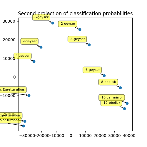
We check that it is different. The following values are the shape of the PCA components. The number of column is the number of dimensions of the outputs of the transfered neural network.

print(pipe.steps[1][1].components_.shape,
      pipe2.steps[1][1].components_.shape)

(2, 1000) (2, 169000)

Graph again.

proj2 = pipe2.transform(X_train)

fig, ax = plt.subplots(1, 1, figsize=(5, 5))
ax.plot(proj2[:, 0], proj2[:, 1], 'o')
ax.set_title("Second projection of classification probabilities")
text = [f"{el[0]:1.0f}-{el[1][0][1]}" for el in climgs]
for label, x, y in zip(text, proj2[:, 0], proj2[:, 1]):
    ax.annotate(
        label, xy=(x, y), xytext=(-10, 10), fontsize=8,
        textcoords='offset points', ha='right', va='bottom',
        bbox=dict(boxstyle='round,pad=0.5', fc='yellow', alpha=0.5),
        arrowprops=dict(arrowstyle='->', connectionstyle='arc3,rad=0'))