Train a linear regression with onnxruntime-training

This example explores how onnxruntime-training can be used to train a simple linear regression using a gradient descent. It compares the results with those obtained by sklearn.linear_model.SGDRegressor

A simple linear regression with scikit-learn

from pprint import pprint
import numpy
import onnx
from pandas import DataFrame
from onnxruntime import (
    InferenceSession, get_device)
from sklearn.datasets import make_regression
from sklearn.model_selection import train_test_split
from sklearn.linear_model import SGDRegressor
from sklearn.neural_network import MLPRegressor
from mlprodict.onnx_conv import to_onnx
from onnxcustom.plotting.plotting_onnx import plot_onnxs
from onnxcustom.utils.orttraining_helper import (
    add_loss_output, get_train_initializer)
from onnxcustom.training.optimizers import OrtGradientOptimizer

X, y = make_regression(n_features=2, bias=2)
X = X.astype(numpy.float32)
y = y.astype(numpy.float32)
X_train, X_test, y_train, y_test = train_test_split(X, y)

lr = SGDRegressor(l1_ratio=0, max_iter=200, eta0=5e-2)
lr.fit(X, y)
print(lr.predict(X[:5]))

[ 53.83746772   6.79334086  86.31569796  73.72210063 -79.5078181 ]

The trained coefficients are:

print("trained coefficients:", lr.coef_, lr.intercept_)

trained coefficients: [67.74134798  7.91162025] [2.00017697]

However this model does not show the training curve. We switch to a sklearn.neural_network.MLPRegressor.

lr = MLPRegressor(hidden_layer_sizes=tuple(),
                  activation='identity', max_iter=200,
                  batch_size=10, solver='sgd',
                  alpha=0, learning_rate_init=1e-2,
                  n_iter_no_change=200,
                  momentum=0, nesterovs_momentum=False)
lr.fit(X, y)
print(lr.predict(X[:5]))

somewhere/workspace/onnxcustom/onnxcustom_UT_39_std/_venv/lib/python3.9/site-packages/sklearn/neural_network/_multilayer_perceptron.py:679: ConvergenceWarning: Stochastic Optimizer: Maximum iterations (200) reached and the optimization hasn't converged yet.
  warnings.warn(
[ 53.842594    6.7937374  86.3236     73.72894   -79.51577  ]

The trained coefficients are:

print("trained coefficients:", lr.coefs_, lr.intercepts_)

trained coefficients: [array([[67.74782 ],
       [ 7.911858]], dtype=float32)] [array([2.0000002], dtype=float32)]

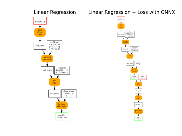
ONNX graph

Training with onnxruntime-training starts with an ONNX graph which defines the model to learn. It is obtained by simply converting the previous linear regression into ONNX.

onx = to_onnx(lr, X_train[:1].astype(numpy.float32), target_opset=15,
              black_op={'LinearRegressor'})

Choosing a loss

The training requires a loss function. By default, it is the square function but it could be the absolute error or include regularization. Function add_loss_output appends the loss function to the ONNX graph.

onx_train = add_loss_output(onx)

plot_onnxs(onx, onx_train,
           title=['Linear Regression',
                  'Linear Regression + Loss with ONNX'])

array([<AxesSubplot: title={'center': 'Linear Regression'}>,
       <AxesSubplot: title={'center': 'Linear Regression + Loss with ONNX'}>],
      dtype=object)

Let’s check inference is working.

sess = InferenceSession(onx_train.SerializeToString(),
                        providers=['CPUExecutionProvider'])
res = sess.run(None, {'X': X_test, 'label': y_test.reshape((-1, 1))})
print(f"onnx loss={res[0][0, 0] / X_test.shape[0]!r}")

onnx loss=2.4012649646465434e-08

Weights

Every initializer is a set of weights which can be trained and a gradient will be computed for it. However an initializer used to modify a shape or to extract a subpart of a tensor does not need training. Let’s remove them from the list of initializer to train.

inits = get_train_initializer(onx)
weights = {k: v for k, v in inits.items() if k != "shape_tensor"}
pprint(list((k, v[0].shape) for k, v in weights.items()))

[('coefficient', (2, 1)), ('intercepts', (1, 1))]

Train on CPU or GPU if available

device = "cuda" if get_device().upper() == 'GPU' else 'cpu'
print(f"device={device!r} get_device()={get_device()!r}")

device='cpu' get_device()='CPU'

Stochastic Gradient Descent

The training logic is hidden in class OrtGradientOptimizer. It follows scikit-learn API (see SGDRegressor. The gradient graph is not available at this stage.

train_session = OrtGradientOptimizer(
    onx_train, list(weights), device=device, verbose=1, learning_rate=1e-2,
    warm_start=False, max_iter=200, batch_size=10,
    saved_gradient="saved_gradient.onnx")

train_session.fit(X, y)

  0%|          | 0/200 [00:00<?, ?it/s]
 16%|#5        | 31/200 [00:00<00:00, 309.89it/s]
 34%|###4      | 68/200 [00:00<00:00, 343.63it/s]
 52%|#####2    | 105/200 [00:00<00:00, 355.36it/s]
 71%|#######1  | 142/200 [00:00<00:00, 360.51it/s]
 90%|########9 | 179/200 [00:00<00:00, 363.87it/s]
100%|##########| 200/200 [00:00<00:00, 357.83it/s]

OrtGradientOptimizer(model_onnx='ir_version...', weights_to_train=['coefficient', 'intercepts'], loss_output_name='loss', max_iter=200, training_optimizer_name='SGDOptimizer', batch_size=10, learning_rate=LearningRateSGD(eta0=0.01, alpha=0.0001, power_t=0.25, learning_rate='invscaling'), value=0.0026591479484724943, device='cpu', warm_start=False, verbose=1, validation_every=20, saved_gradient='saved_gradient.onnx', sample_weight_name='weight')

And the trained coefficient are…

state_tensors = train_session.get_state()
pprint(["trained coefficients:", state_tensors])
print("last_losses:", train_session.train_losses_[-5:])

min_length = min(len(train_session.train_losses_), len(lr.loss_curve_))
df = DataFrame({'ort losses': train_session.train_losses_[:min_length],
                'skl losses': lr.loss_curve_[:min_length]})
df.plot(title="Train loss against iterations")

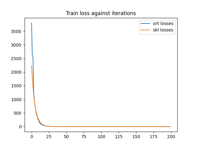
['trained coefficients:',
 {'coefficient': array([[67.74761  ],
       [ 7.9118924]], dtype=float32),
  'intercepts': array([[1.9999774]], dtype=float32)}]
last_losses: [1.8183808e-07, 1.3479456e-07, 1.2890612e-07, 1.6501485e-07, 1.506005e-07]

<AxesSubplot: title={'center': 'Train loss against iterations'}>

the training graph looks like the following…

with open("saved_gradient.onnx.training.onnx", "rb") as f:
    graph = onnx.load(f)
    for inode, node in enumerate(graph.graph.node):
        if '' in node.output:
            for i in range(len(node.output)):
                if node.output[i] == "":
                    node.output[i] = "n%d-%d" % (inode, i)

plot_onnxs(graph, title='Training graph')

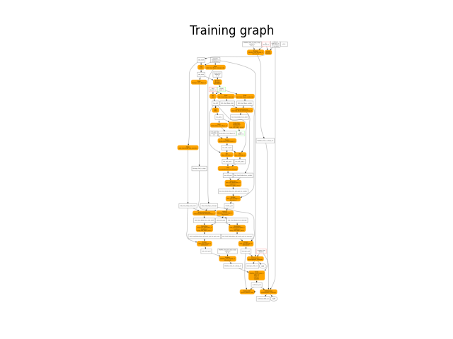
<AxesSubplot: title={'center': 'Training graph'}>

The convergence speed is not the same but both gradient descents do not update the gradient multiplier the same way. onnxruntime-training does not implement any gradient descent, it just computes the gradient. That’s the purpose of OrtGradientOptimizer. Next example digs into the implementation details.

# import matplotlib.pyplot as plt
# plt.show()