Clustering

Le clustering est une méthode non supervisée qui vise à répartir les données selon leur similarité dans des clusters. L’inconnu de ce type de problèmes est le nombre de clusters.

Principe

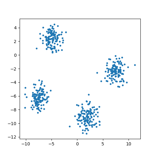
On commence par générer un nuage de points artificiel.

import numpy
from sklearn.metrics import silhouette_samples, silhouette_score
from sklearn.cluster import KMeans
import matplotlib.pyplot as plt
from sklearn.datasets import make_blobs
X, Y = make_blobs(n_samples=500, n_features=2, centers=4)

On représente ces données.

fig, ax = plt.subplots(1, 1, figsize=(5, 5))
ax.plot(X[:, 0], X[:, 1], '.')

[<matplotlib.lines.Line2D object at 0x7f5f36dedc70>]

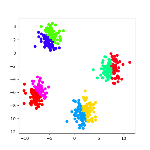
On utilise un algorithme très utilisé : KMeans.

km = KMeans()
km.fit(X)

/usr/local/lib/python3.9/site-packages/sklearn/cluster/_kmeans.py:870: FutureWarning: The default value of `n_init` will change from 10 to 'auto' in 1.4. Set the value of `n_init` explicitly to suppress the warning
  warnings.warn(

KMeans()

In a Jupyter environment, please rerun this cell to show the HTML representation or trust the notebook.
On GitHub, the HTML representation is unable to render, please try loading this page with nbviewer.org.

L’optimisation du modèle produit autant de points que de clusters.

print(km.cluster_centers_)

[[ 2.81219206 -8.66796052]
 [-5.39610266  1.66554465]
 [-7.93921872 -6.77276865]
 [ 6.77222059 -2.35684426]
 [ 1.13637447 -9.37453472]
 [-4.45946923  2.99653347]
 [-6.93449447 -5.51329065]
 [ 8.44625973 -2.46233653]]

On dessine le résultat en choisissant une couleur différente pour chaque cluster.

cmap = plt.cm.get_cmap("hsv", km.cluster_centers_.shape[0])
fig, ax = plt.subplots(1, 1, figsize=(5, 5))
colors = [cmap(i) for i in km.fit_predict(X)]
ax.scatter(X[:, 0], X[:, 1], c=colors)

somewhere/workspace/papierstat/papierstat_UT_39_std/_doc/examples/ml_basic/plot_clustering.py:53: MatplotlibDeprecationWarning: The get_cmap function was deprecated in Matplotlib 3.7 and will be removed two minor releases later. Use ``matplotlib.colormaps[name]`` or ``matplotlib.colormaps.get_cmap(obj)`` instead.
  cmap = plt.cm.get_cmap("hsv", km.cluster_centers_.shape[0])
/usr/local/lib/python3.9/site-packages/sklearn/cluster/_kmeans.py:870: FutureWarning: The default value of `n_init` will change from 10 to 'auto' in 1.4. Set the value of `n_init` explicitly to suppress the warning
  warnings.warn(

<matplotlib.collections.PathCollection object at 0x7f5f36c2f610>

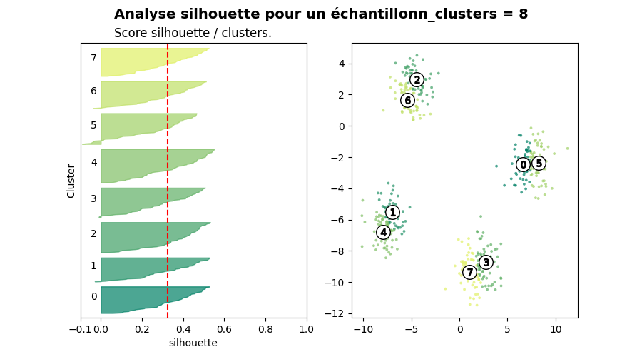
Autre graphe et métrique silhouette

Inspiré de Selecting the number of clusters with silhouette analysis on KMeans clustering. Il s’agit de représenter la dispersion au sein de chaque cluster. Sont-ils concentrés autour d’un point ou plutôt regroupés parce que loin de tout ? On commence par calculer le score silhouette puis à prendre un échantillon aléatoire sous peine d’avoir un graphique surchargé.

cluster_labels = km.fit_predict(X)
silhouette_avg = silhouette_score(X, cluster_labels)
sample_silhouette_values = silhouette_samples(X, cluster_labels)
centers = km.cluster_centers_
n_clusters = centers.shape[0]

/usr/local/lib/python3.9/site-packages/sklearn/cluster/_kmeans.py:870: FutureWarning: The default value of `n_init` will change from 10 to 'auto' in 1.4. Set the value of `n_init` explicitly to suppress the warning
  warnings.warn(

On dessine.

try:
    from matplotlib.cm import spectral as color_map
except ImportError:
    from matplotlib.cm import summer as color_map

fig, (ax1, ax2) = plt.subplots(1, 2)
fig.set_size_inches(9, 5)

ax1.set_xlim([-0.1, 1])
ax1.set_ylim([0, len(X) + (km.n_clusters + 1) * 10])

y_lower = 10
for i in range(n_clusters):
    ith_cluster_silhouette_values = sample_silhouette_values[cluster_labels == i]
    ith_cluster_silhouette_values.sort()

    size_cluster_i = ith_cluster_silhouette_values.shape[0]
    y_upper = y_lower + size_cluster_i

    color = color_map(float(i) / n_clusters)
    ax1.fill_betweenx(numpy.arange(y_lower, y_upper),
                      0, ith_cluster_silhouette_values,
                      facecolor=color, edgecolor=color, alpha=0.7)

    ax1.text(-0.05, y_lower + 0.5 * size_cluster_i, str(i))
    y_lower = y_upper + 10

ax1.set_title("Score silhouette / clusters.")
ax1.set_xlabel("silhouette")
ax1.set_ylabel("Cluster")

ax1.axvline(x=silhouette_avg, color="red", linestyle="--")

ax1.set_yticks([])
ax1.set_xticks([-0.1, 0, 0.2, 0.4, 0.6, 0.8, 1])

colors = color_map(cluster_labels.astype(float) / n_clusters)
ax2.scatter(X[:, 0], X[:, 1], marker='.', s=30,
            lw=0, alpha=0.7, c=colors, edgecolor='k')
ax2.scatter(centers[:, 0], centers[:, 1], marker='o',
            c="white", alpha=1, s=200, edgecolor='k')

for i, c in enumerate(centers):
    ax2.scatter(c[0], c[1], marker='$%d$' % i, alpha=1,
                s=50, edgecolor='k')

plt.suptitle(("Analyse silhouette pour un échantillon"
              "n_clusters = %d" % n_clusters),
             fontsize=14, fontweight='bold')

findfont: Font family ['STIXGeneral'] not found. Falling back to DejaVu Sans.
findfont: Font family ['STIXGeneral'] not found. Falling back to DejaVu Sans.
findfont: Font family ['STIXGeneral'] not found. Falling back to DejaVu Sans.
findfont: Font family ['STIXNonUnicode'] not found. Falling back to DejaVu Sans.
findfont: Font family ['STIXNonUnicode'] not found. Falling back to DejaVu Sans.
findfont: Font family ['STIXNonUnicode'] not found. Falling back to DejaVu Sans.
findfont: Font family ['STIXSizeOneSym'] not found. Falling back to DejaVu Sans.
findfont: Font family ['STIXSizeTwoSym'] not found. Falling back to DejaVu Sans.
findfont: Font family ['STIXSizeThreeSym'] not found. Falling back to DejaVu Sans.
findfont: Font family ['STIXSizeFourSym'] not found. Falling back to DejaVu Sans.
findfont: Font family ['STIXSizeFiveSym'] not found. Falling back to DejaVu Sans.
findfont: Font family ['cmsy10'] not found. Falling back to DejaVu Sans.
findfont: Font family ['cmr10'] not found. Falling back to DejaVu Sans.
findfont: Font family ['cmtt10'] not found. Falling back to DejaVu Sans.
findfont: Font family ['cmmi10'] not found. Falling back to DejaVu Sans.
findfont: Font family ['cmb10'] not found. Falling back to DejaVu Sans.
findfont: Font family ['cmss10'] not found. Falling back to DejaVu Sans.
findfont: Font family ['cmex10'] not found. Falling back to DejaVu Sans.
findfont: Font family ['DejaVu Sans Display'] not found. Falling back to DejaVu Sans.

Text(0.5, 0.98, 'Analyse silhouette pour un échantillonn_clusters = 8')