Saisonnalités, changement de régime, COVID en France#

Links: notebook, html, PDF, python, slides, GitHub

On s’intéresse aux séries temporelles de l’épidémie du COVID en France récupérées depuis data.gouv.fr : Chiffres-clés concernant l’épidémie de COVID19 en France.

from jyquickhelper import add_notebook_menu
add_notebook_menu()

%matplotlib inline

Données #

from pandas import DataFrame, read_csv, to_datetime
df = read_csv("https://www.data.gouv.fr/en/datasets/r/0b66ca39-1623-4d9c-83ad-5434b7f9e2a4")
df.tail()

c:python387_x64libsite-packagesIPythoncoreinteractiveshell.py:3146: DtypeWarning: Columns (17,18) have mixed types.Specify dtype option on import or set low_memory=False.
  has_raised = await self.run_ast_nodes(code_ast.body, cell_name,

	date	granularite	maille_code	maille_nom	cas_confirmes	cas_ehpad	cas_confirmes_ehpad	cas_possibles_ehpad	deces	deces_ehpad	reanimation	hospitalises	nouvelles_hospitalisations	nouvelles_reanimations	gueris	depistes	source_nom	source_url	source_archive	source_type
43080	2021-02-10	region	REG-75	Nouvelle-Aquitaine	NaN	NaN	NaN	NaN	2510.0	NaN	213.0	1524.0	78.0	20.0	10227.0	NaN	OpenCOVID19-fr	NaN	NaN	opencovid19-fr
43081	2021-02-10	region	REG-76	Occitanie	NaN	NaN	NaN	NaN	2882.0	NaN	276.0	1886.0	121.0	25.0	12801.0	NaN	OpenCOVID19-fr	NaN	NaN	opencovid19-fr
43082	2021-02-10	region	REG-84	Auvergne-Rhône-Alpes	NaN	NaN	NaN	NaN	8453.0	NaN	400.0	3699.0	213.0	42.0	34579.0	NaN	OpenCOVID19-fr	NaN	NaN	opencovid19-fr
43083	2021-02-10	region	REG-93	Provence-Alpes-Côte d'Azur	NaN	NaN	NaN	NaN	5010.0	NaN	438.0	3581.0	240.0	33.0	24080.0	NaN	OpenCOVID19-fr	NaN	NaN	opencovid19-fr
43084	2021-02-10	region	REG-94	Corse	NaN	NaN	NaN	NaN	133.0	NaN	7.0	58.0	4.0	3.0	587.0	NaN	OpenCOVID19-fr	NaN	NaN	opencovid19-fr

# Il y a une date 2020-11_11
df['date'] = to_datetime(df['date'].apply(lambda s: s.replace("_", "-")))

gr = df[["date", "cas_confirmes"]].groupby("date").sum().sort_index()
gr.tail()

	cas_confirmes
date
2021-02-06	3317333.0
2021-02-07	3337048.0
2021-02-08	3341365.0
2021-02-09	3360235.0
2021-02-10	3385622.0

gr['cas_confirmes'].plot(figsize=(14, 4), grid=True, title="Cas positifs");

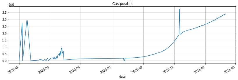
Il y a des petits problèmes de données… On corrige de façon automatique ou à la main… Etant donné que les données n’étaient pas fiables avant juin 2020 car pas assez de tests, on commence la série en septembre 2020. Il ne reste donc plus qu’une date un peu problématique, le 11 novembre.

from datetime import datetime
gr.loc[(gr.index >= datetime(2020, 11, 5)) & (gr.index <= datetime(2020, 11, 15)), 'cas_confirmes'].plot(
    figsize=(14, 2), grid=True, title="Cas positifs");

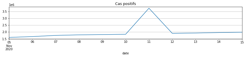
gr.loc[datetime(2020, 11, 11), 'cas_confirmes'] = (
    gr.loc[datetime(2020, 11, 10), 'cas_confirmes'] + gr.loc[datetime(2020, 11, 12), 'cas_confirmes']) / 2

gr.loc[gr.index >= datetime(2020, 9, 1), 'cas_confirmes'].plot(figsize=(14, 4), grid=True, title="Cas positifs");

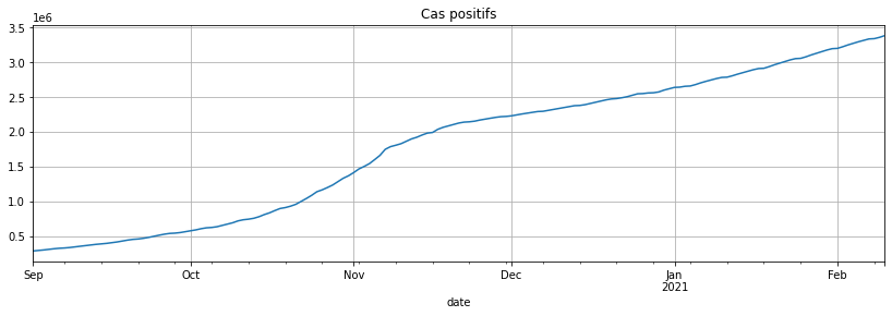
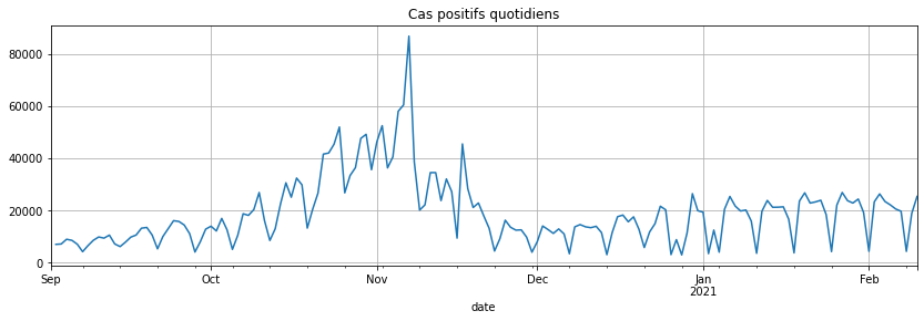
C’est mieux. On regarde la série différenciée :

covsept = gr.loc[gr.index >= datetime(2020, 9, 1), 'cas_confirmes']
covsept.diff().plot(figsize=(14, 4), grid=True, title="Cas positifs quotidiens");

Changements de régimes #

fbprophet quand ça marche #

from fbprophet import Prophet
from fbprophet.plot import add_changepoints_to_plot
try:
    m = Prophet(changepoint_prior_scale=0.5)
    fig = m.plot(covsept)
    a = add_changepoints_to_plot(fig.gca(), m, covsept)
except AttributeError as e:
    print(e)
    # Sur Windows, fbprophet est compliqué à installer.
    # J'ai abandonné. C'est plus simple sous Linux.

Importing plotly failed. Interactive plots will not work.

'Prophet' object has no attribute 'stan_backend'

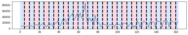
On passe à un autre module. Il compare localement la moyenne de la série à la série elle-même. Sur ce type de série avec une périodicité, ça ne marche pas très bien.

Ecart à la moyenne #

import ruptures

signal = covsept.diff().values

algo = ruptures.Pelt(model="rbf").fit(signal)
result = algo.predict(pen=10)

ruptures.display(signal, result, result);

import numpy
signal = covsept.diff().values
X = numpy.arange(signal.shape[0]).reshape(-1, 1).astype(signal.dtype)[1:]
y = signal[1:]
X.shape, y.shape

((162, 1), (162,))

Cuisine maison #

Donc je suis finalement passé à quelque chose que j’ai codé : un arbre de régression mais donc chaque feuille est une régression linéaire et non une constante. Ca manque un peu de théorie mais rien n’empêche d’être un peu inventif :PiecewiseTreeRegressor.

from mlinsights.mlmodel import PiecewiseTreeRegressor
ptr = PiecewiseTreeRegressor(min_samples_leaf=14)
ptr.fit(X, y)

C:xavierdupre__home_github_forkscikit-learnsklearntree_classes.py:335: FutureWarning: The parameter 'X_idx_sorted' is deprecated and has no effect. It will be removed in 1.1 (renaming of 0.26). You can suppress this warning by not passing any value to the 'X_idx_sorted' parameter.
  warnings.warn(

PiecewiseTreeRegressor(min_samples_leaf=14)

import matplotlib.pyplot as plt
fig, ax = plt.subplots(1, 1, figsize=(14, 4))
ax.plot(X, y)
ax.plot(X, ptr.predict(X))
ax.set_title("Changement de régime estimer avec des arbres de régression");

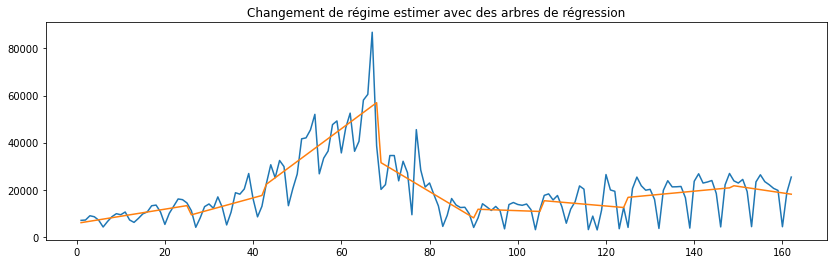
L’épidémie progresse de façon explonentielle. Il vaudrait sans doute mieux étudier le logarithme de la série différenciée.

ptrl = PiecewiseTreeRegressor(min_samples_leaf=14)
ly = numpy.log(y)
ptrl.fit(X, ly)

fig, ax = plt.subplots(1, 1, figsize=(14, 4))
ax.plot(X, ly)
ax.plot(X, ptrl.predict(X))
ax.set_title("Changement de régime estimer avec des arbres de régression"
             "\nversion logarithmique");

C:xavierdupre__home_github_forkscikit-learnsklearntree_classes.py:335: FutureWarning: The parameter 'X_idx_sorted' is deprecated and has no effect. It will be removed in 1.1 (renaming of 0.26). You can suppress this warning by not passing any value to the 'X_idx_sorted' parameter.
  warnings.warn(

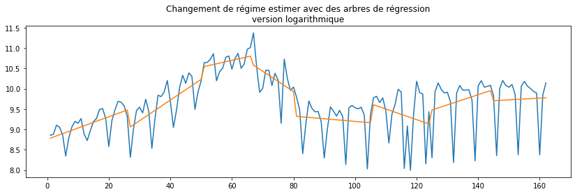
C’est un petit peu mieux. Cette méthode s’applique surtout à la tendance des séries contrairement à la méthode suivante plus approprié pour segmenter les résidus.

Gaussian Hidden Markov Model #

Qu’est-ce ?

from hmmlearn.hmm import GaussianHMM
model = GaussianHMM(n_components=3, covariance_type="diag", n_iter=1000)
model.fit(ly.reshape(-1, 1))
model

GaussianHMM(n_components=3, n_iter=1000)

hidden_states = model.predict(X)
dates = covsept.index[1:]
set(hidden_states)

{1}

Le model n’arrive à rien sauf à prédire une valeur constante.

fig, axs = plt.subplots(model.n_components, sharex=True, sharey=True, figsize=(14, 6))
for i, ax in enumerate(axs):
    mask = hidden_states == i
    ax.plot(X[mask], ly[mask], ".-")
    ax.set_title("{0}th hidden state".format(i))
    ax.grid(True)

Ca ne donne rien car la saisonnalité l’emporte sur le reste.

Les modules classiques #

Saisonnalité #

Saisonnalité et moyennes mobiles #

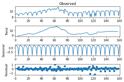
from statsmodels.tsa.seasonal import seasonal_decompose
res = seasonal_decompose(ly, freq=7)
res.plot();

<ipython-input-21-96d157ac9bae>:2: FutureWarning: the 'freq'' keyword is deprecated, use 'period' instead
  res = seasonal_decompose(ly, freq=7)

res.resid[:10]

array([        nan,         nan,         nan,  0.07542526, -0.02752109,
        0.3475441 , -0.11152892, -0.15329366, -0.04130195, -0.09907971])

Quelque chose qui n’a pas beaucoup de sens #

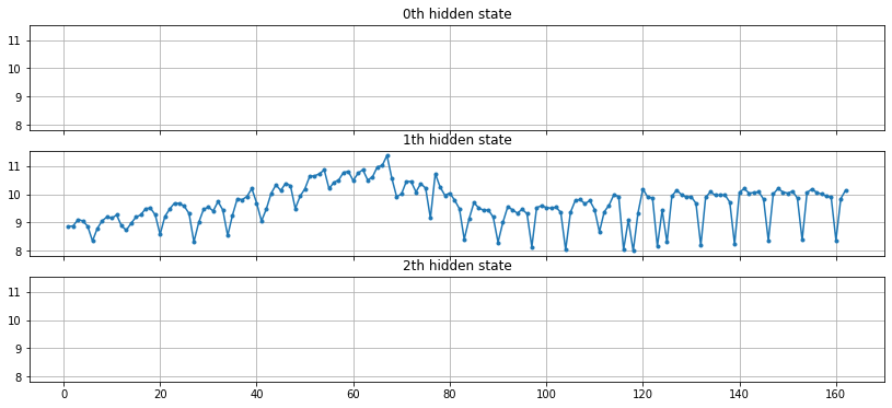
model = GaussianHMM(n_components=3, covariance_type="diag", n_iter=1000)
ry = res.trend[3:-3]  # on enlève les nan
model.fit(ry.reshape(-1, 1))
hidden_states = model.predict(ry.reshape(-1, 1))
set(hidden_states)

{0, 1, 2}

fig, axs = plt.subplots(model.n_components, sharex=True, sharey=True, figsize=(14, 6))
for i, ax in enumerate(axs):
    mask = hidden_states == i
    ax.plot(numpy.arange(0, ry.shape[0])[mask], ry[mask], ".-")
    ax.set_title("{0}th hidden state".format(i))
    ax.grid(True)

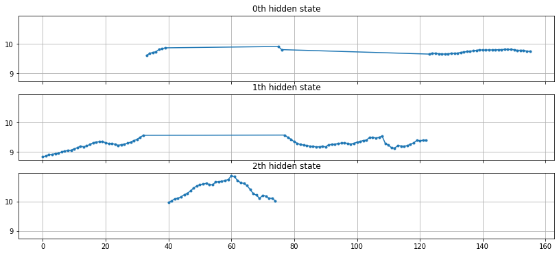
Si le modèle gaussien a l’air de fonctionner sur la série tendancielle (hors saisonnalité), il est plutôt utilisé pour segmenter selon la loi des résidus. Sur chaque segments, la série peut être approchée par une loi normale de moyenne et variance différentes.

model.means_, model.covars_

(array([[ 9.75077896],
        [ 9.26327355],
        [10.40300854]]),
 array([[[0.00506213]],
        [[0.02444731]],
        [[0.07163662]]]))

ExponentialSmoothing #

Le lissage exponentiel consite à modéliser la série comme suit :

$\begin{array}{rcl} s_0 &=& y_0 \\ s_t &=& \alpha y_t + (1-\alpha) s_{t-1} \text{ pour } t > 0 \end{array}$

Ou :

$\begin{array}{rcl} s_1 &=& y_1 \\ \sigma_1 &=& y_1 - y_0 \\ s_t &=& \alpha y_t + (1-\alpha) (s_{t-1} + \sigma_{t-1}) \text{ pour } t > 1 \\ \sigma_t &=& \beta (s_t - s_{t-1}) + (1-\beta) \sigma_{t-1} \text{ pour } t > 1 \end{array}$

Ou plus complexe avec Holt Winters:

$\begin{array}{rcl} s_0 &=& y_0 \\ s_t &=& \alpha (y_t - c_{t - L}) + (1-\alpha) (s_{t-1} + b_{t-1}) \\ b_t &=& \beta(s_t - s_{t-1}) + (1-\beta)b_{t-1} \\ c_t &=& \gamma (y_t - s_{t-1} - b_{t-1}) + (1-\gamma)c_{t-L} \end{array}$

from statsmodels.tsa.holtwinters import ExponentialSmoothing
fit1 = ExponentialSmoothing(y, seasonal_periods=7, trend='add', seasonal='add').fit(use_boxcox=True)
fit2 = ExponentialSmoothing(y, seasonal_periods=7, trend='add', seasonal='mul').fit(use_boxcox=True)
fit3 = ExponentialSmoothing(y, seasonal_periods=7, trend='add', seasonal='add', damped=True).fit(use_boxcox=True)
fit4 = ExponentialSmoothing(y, seasonal_periods=7, trend='add', seasonal='mul', damped=True).fit(use_boxcox=True)

c:python387_x64libsite-packagesstatsmodelstsaholtwintersmodel.py:427: FutureWarning: After 0.13 initialization must be handled at model creation
  warnings.warn(
c:python387_x64libsite-packagesstatsmodelstsaholtwintersmodel.py:1112: FutureWarning: Setting use_boxcox during fit has been deprecated and will be removed after 0.13. It must be set during model initialization.
  warnings.warn(
<ipython-input-26-0a978064fcad>:4: FutureWarning: the 'damped'' keyword is deprecated, use 'damped_trend' instead
  fit3 = ExponentialSmoothing(y, seasonal_periods=7, trend='add', seasonal='add', damped=True).fit(use_boxcox=True)
<ipython-input-26-0a978064fcad>:5: FutureWarning: the 'damped'' keyword is deprecated, use 'damped_trend' instead
  fit4 = ExponentialSmoothing(y, seasonal_periods=7, trend='add', seasonal='mul', damped=True).fit(use_boxcox=True)

fit1.summary()

ExponentialSmoothing Model Results
Dep. Variable:	endog	No. Observations:	162
Model:	ExponentialSmoothing	SSE	7985315446.470
Optimized:	True	AIC	2891.550
Trend:	Additive	BIC	2925.514
Seasonal:	Additive	AICC	2894.010
Seasonal Periods:	7	Date:	Wed, 10 Feb 2021
Box-Cox:	True	Time:	23:00:39
Box-Cox Coeff.:	0.19415

	coeff	code	optimized
smoothing_level	0.2185487	alpha	True
smoothing_trend	0.1681336	beta	True
smoothing_seasonal	0.2405703	gamma	True
initial_level	29.375329	l.0	True
initial_trend	0.1857434	b.0	True
initial_seasons.0	-5.9555579	s.0	True
initial_seasons.1	-5.4784169	s.1	True
initial_seasons.2	-5.2732824	s.2	True
initial_seasons.3	-5.0576235	s.3	True
initial_seasons.4	-6.8353828	s.4	True
initial_seasons.5	-10.316491	s.5	True
initial_seasons.6	-7.6978206	s.6	True

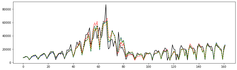
fig, ax = plt.subplots(1, 1, figsize=(14, 4))
ax.plot(y, 'b', color='black', label="Cas positifs")
ax.plot(fit1.fittedvalues, '--', color='red')
ax.plot(fit2.fittedvalues, '--', color='blue')
ax.plot(fit3.fittedvalues, '--', color='orange')
ax.plot(fit4.fittedvalues, '--', color='green');

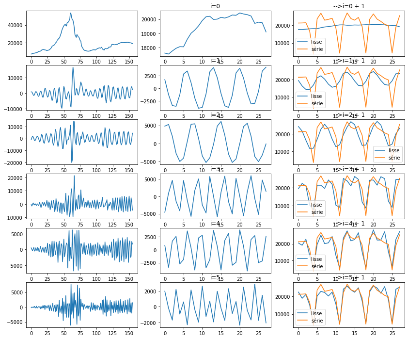
Single Spectrum Analysis (SSA)#

Le module `pyts <>`__ ne fonctionnait pas pour moi. Je suis alors le notebook Single Spectrum Analysis (SSA).

def lagged_ts(serie, lag):
    dim = serie.shape[0]
    res = numpy.zeros((dim - lag + 1, lag))
    for i in range(lag):
        res[:, i] = serie[i:dim-lag+i+1]
    return res

lagged_ts(y, 3)[:5]

array([[7017., 7157., 8975.],
       [7157., 8975., 8550.],
       [8975., 8550., 7071.],
       [8550., 7071., 4203.],
       [7071., 4203., 6544.]])

n_lag = 7
lag = lagged_ts(y, n_lag)
u, s, vh = svd(lag)
u.shape

(156, 156)

from numpy.linalg import svd
np = 6
fig, ax = plt.subplots(np, 3, figsize=(14, np*2))
for n in range(np):
    i = n
    d = numpy.zeros((u.shape[0], n_lag))
    d[i, i] = s[i]
    X2 = u @ d @ vh
    pos = 0 #X2.shape[1] - 1

    # série reconstruites avec un axe
    ax[n, 0].plot(X2[:,pos])
    ax[n, 1].set_title("i=%d" % i)
    ax[n, 1].plot(X2[-29:-1:,pos])

    d = numpy.zeros((u.shape[0], n_lag))
    d[:i+1, :i+1] = numpy.diag(s[:i+1])
    X2 = u @ d @ vh
    ax[n, 2].plot(X2[-29:-1,pos], label="lisse")
    ax[n, 2].plot(y[-28:], label="série")
    ax[n, 2].set_title("-->i=%d + 1" % i)
    ax[n, 2].legend()

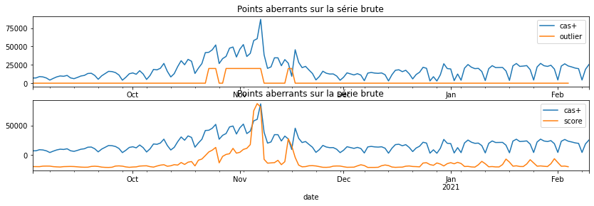
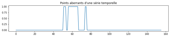
Points aberrants #

d = numpy.zeros((u.shape[0], n_lag))
for i in range(0, d.shape[1]):
    d[i, i] = s[i]
X2 = u @ d @ vh

from sklearn.covariance import EllipticEnvelope
env = EllipticEnvelope(support_fraction=0.9)
env.fit(X2[:,:n_lag // 2])
out = env.predict(X2[:,:n_lag // 2])

fig, ax = plt.subplots(1, 1, figsize=(12,2))
ax.plot((1 - out)/2, "-")
ax.set_title("Points aberrants d'une série temporelle");

fig, ax = plt.subplots(2, 1, figsize=(14,4))
outp = env.decision_function(X2[:,:n_lag // 2])
dfy = DataFrame(data=y, index=dates, columns=["cas+"])
dfy['outlier'] = dfy['score'] = numpy.nan
dfy.iloc[:-n_lag+1, 1] = (1 - out)*1e4
dfy.iloc[:-n_lag+1, 2] = -outp*1e3
dfy[['cas+', 'outlier']].plot(ax=ax[0])
ax[0].set_title("Points aberrants sur la série brute");
dfy[['cas+', 'score']].plot(ax=ax[1])
ax[1].set_title("Points aberrants sur la série brute");

Liens

Contenu

Information

Sujet précédent

Sujet suivant