Interprétation de la note d’un vin#
Links: notebook, html, PDF, python, slides, GitHub
Le notebook explore différentes façons d’interpréter la prédiction de la note d’un vin.
from jyquickhelper import add_notebook_menu
add_notebook_menu()
%matplotlib inline
Un aperçu des données#
from papierstat.datasets import load_wines_dataset
df = load_wines_dataset()
X = df.drop(['quality', 'color'], axis=1)
y = df['quality']
df.head()
| fixed_acidity | volatile_acidity | citric_acid | residual_sugar | chlorides | free_sulfur_dioxide | total_sulfur_dioxide | density | pH | sulphates | alcohol | quality | color | |
|---|---|---|---|---|---|---|---|---|---|---|---|---|---|
| 0 | 7.4 | 0.70 | 0.00 | 1.9 | 0.076 | 11.0 | 34.0 | 0.9978 | 3.51 | 0.56 | 9.4 | 5 | red |
| 1 | 7.8 | 0.88 | 0.00 | 2.6 | 0.098 | 25.0 | 67.0 | 0.9968 | 3.20 | 0.68 | 9.8 | 5 | red |
| 2 | 7.8 | 0.76 | 0.04 | 2.3 | 0.092 | 15.0 | 54.0 | 0.9970 | 3.26 | 0.65 | 9.8 | 5 | red |
| 3 | 11.2 | 0.28 | 0.56 | 1.9 | 0.075 | 17.0 | 60.0 | 0.9980 | 3.16 | 0.58 | 9.8 | 6 | red |
| 4 | 7.4 | 0.70 | 0.00 | 1.9 | 0.076 | 11.0 | 34.0 | 0.9978 | 3.51 | 0.56 | 9.4 | 5 | red |
from sklearn.model_selection import train_test_split
X_train, X_test, y_train, y_test = train_test_split(X, y, test_size=0.9)
from sklearn.ensemble import HistGradientBoostingRegressor
rf = HistGradientBoostingRegressor(max_iter=10)
rf.fit(X_train, y_train)
HistGradientBoostingRegressor(max_iter=10)
from sklearn.metrics import r2_score
r2_score(y_test, rf.predict(X_test))
0.24727950503706164
X_train.shape, len(rf.feature_names_in_)
((649, 11), 11)
rf.feature_names_in_
array(['fixed_acidity', 'volatile_acidity', 'citric_acid',
       'residual_sugar', 'chlorides', 'free_sulfur_dioxide',
       'total_sulfur_dioxide', 'density', 'pH', 'sulphates', 'alcohol'],
      dtype=object)
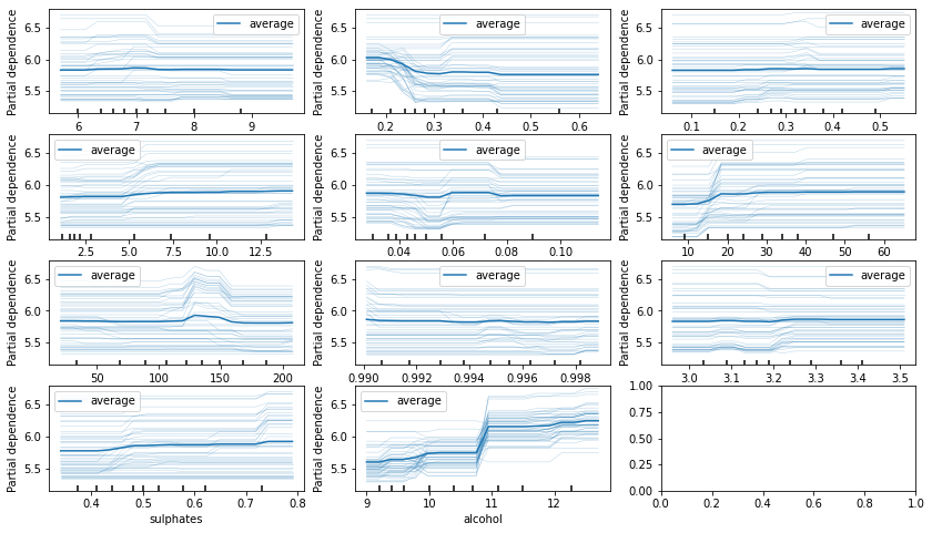
Partial dependance#
L’idée est d’observer comment varie les prédictions en faisant évoluer
une variable et en laissant les autres fixes. Concrètement, pour la
variable j et une observations
 , on construit une autre
variable
, on construit une autre
variable  où la variable j est remplacé par une autre prise chez une autre
observation.
où la variable j est remplacé par une autre prise chez une autre
observation.
import matplotlib.pyplot as plt
from sklearn.inspection import (
    partial_dependence, PartialDependenceDisplay)

fig, ax = plt.subplots(4, 3, figsize=(14, 8))
display = PartialDependenceDisplay.from_estimator(
    rf, X_train, list(rf.feature_names_in_), kind="both",
    subsample=50, n_jobs=3, grid_resolution=20,
    random_state=0, ax=ax.ravel()[:11])
LIME#
Pour résumer, l’approche LIME consiste à approximer les prédictions d’un modèle compliqué par un modèle plus simple comme un modèle linéaire. Comme le modèle simple ne peut être aussi précis que le modèle compliqué, il est estimé au voisinage de chaque observation dont on cherche à expliquer la prédiction.
import warnings
from interpret import show
from interpret.blackbox import LimeTabular

with warnings.catch_warnings():
    warnings.simplefilter('ignore')

    lime = LimeTabular(predict_fn=rf.predict, data=X_train,
                       feature_names=list(rf.feature_names_in_))
    lime_local = lime.explain_local(X_test[:5], y_test[:5])

show(lime_local)
Shap#
La méthode précédente ne fonctionne pas si les variables sont corrélées. L’idée de Shap est de mesurer ce qu’apporte une variable en apprenant un modèle avec et sans. Ce faisant, il faut le faire sur tous les combinaisons possibles de variables. C’est très long. Voici un algorithme approché tiré de ce livre :
Approximate Shapley estimation for single feature value:
Output: Shapley value for the value of the j-th feature
Required: Number of iterations M, instance of interest x, feature index j, data matrix X, and machine learning model f
For all m = 1,…,M:
Draw random instance z from the data matrix X
Choose a random permutation o of the feature values
Order instance x:

Order instance x:

Construct two new instances:
With j:

Without j:

Compute marginal contribution

Compute Shapley value as the average:

from interpret.blackbox import ShapKernel

shap = ShapKernel(predict_fn=rf.predict, data=X_train,
                  feature_names=list(rf.feature_names_in_))
shap_local = shap.explain_local(X_test[:5], y_test[:5])
X does not have valid feature names, but HistGradientBoostingRegressor was fitted with feature names
X does not have valid feature names, but HistGradientBoostingRegressor was fitted with feature names
Using 1299 background data samples could cause slower run times. Consider using shap.sample(data, K) or shap.kmeans(data, K) to summarize the background as K samples.
0%| | 0/5 [00:00<?, ?it/s]
X does not have valid feature names, but HistGradientBoostingRegressor was fitted with feature names
X does not have valid feature names, but HistGradientBoostingRegressor was fitted with feature names
X does not have valid feature names, but HistGradientBoostingRegressor was fitted with feature names
X does not have valid feature names, but HistGradientBoostingRegressor was fitted with feature names
X does not have valid feature names, but HistGradientBoostingRegressor was fitted with feature names
X does not have valid feature names, but HistGradientBoostingRegressor was fitted with feature names
X does not have valid feature names, but HistGradientBoostingRegressor was fitted with feature names
X does not have valid feature names, but HistGradientBoostingRegressor was fitted with feature names
X does not have valid feature names, but HistGradientBoostingRegressor was fitted with feature names
X does not have valid feature names, but HistGradientBoostingRegressor was fitted with feature names
X does not have valid feature names, but HistGradientBoostingRegressor was fitted with feature names
show(shap_local)