ONNX in a torch function

The ONNX graph used in this example is not really interesting but it shows how to create a custom autograd function following torch API (Extending Pytorch). Methods forward and backward are implemented with ONNX and onnxruntime-training.

The ONNX Graph

import pprint
import logging
import numpy
from pandas import DataFrame
import matplotlib.pyplot as plt
from skl2onnx.common.data_types import FloatTensorType
from skl2onnx.algebra.onnx_ops import (
    OnnxSigmoid, OnnxMatMul, OnnxAdd)
from tqdm import tqdm
from mlprodict.onnx_tools.onnx_manipulations import onnx_rename_names
from mlprodict.plotting.plotting_onnx import plot_onnx
import torch
from deeponnxcustom.onnxtorch.torchort import TorchOrtFactory


def from_numpy(v, device=None, requires_grad=False):
    """
    Convers a numpy array into a torch array and
    sets *device* and *requires_grad*.
    """
    v = torch.from_numpy(v)
    if device is not None:
        v = v.to(device)
    v.requires_grad_(requires_grad)
    return v


def create_onnx_graph(N, d_in=3, d_out=2, n_loops=1, opv=14):
    """
    Returns a weird ONNX graph and its weights.
    """
    var = [('X', FloatTensorType([N, d_in]))]

    sum_node = None
    weights_values = []
    for i in range(n_loops):
        cst = numpy.random.randn(d_in, 1).astype(numpy.float32) / (i + 1)
        weights_values.append(cst)
        mul = OnnxMatMul(var[0], cst, op_version=opv)
        tanh = OnnxSigmoid(mul, op_version=opv)
        if sum_node is None:
            sum_node = tanh
        else:
            sum_node = OnnxAdd(sum_node, tanh, op_version=opv)

    cst_mul = numpy.random.randn(1, d_out).astype(numpy.float32)
    weights_values.append(cst_mul)
    mul = OnnxMatMul(sum_node, cst_mul, op_version=opv)

    cst_add = numpy.random.randn(1, d_out).astype(numpy.float32)
    weights_values.append(cst_add)
    final = OnnxAdd(mul, cst_add, op_version=opv, output_names=['Y'])

    onx = final.to_onnx(
        var, target_opset=opv, outputs=[('Y', FloatTensorType())])

    weights_name = [i.name for i in onx.graph.initializer]
    new_names = ['W%03d' % i for i in range(len(weights_name))]
    onx = onnx_rename_names(onx, replace=dict(zip(weights_name, new_names)))
    weights = list(zip(new_names, weights_values))
    return onx, weights

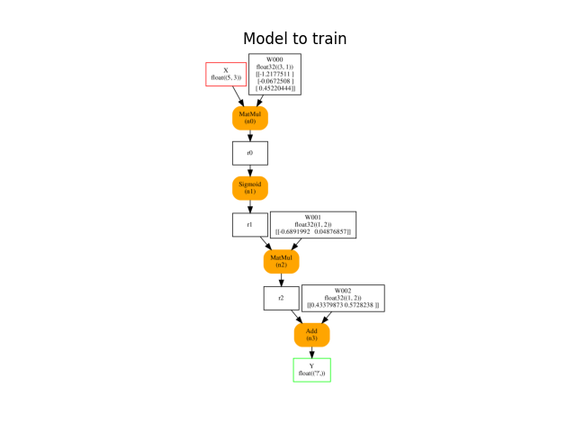
Let’s see how it looks like.

N, d_in, d_out = 5, 3, 2
enable_logging = False
onx, weights = create_onnx_graph(N)

with open("plot_torch_ort.onnx", "wb") as f:
    f.write(onx.SerializeToString())
print("weights to train:", [(w[0], w[1].shape) for w in weights])

ax = plot_onnx(onx)
ax.set_title("Model to train")

Out:

weights to train: [('W000', (3, 1)), ('W001', (1, 2)), ('W002', (1, 2))]

Text(0.5, 1.0, 'Model to train')

Wraps ONNX as a torch.autograd.Function

Class TorchOrtFactory uses onnxruntime-training to build the gradient with ONNX, add calls it following this logic:

class CustomClass(torch.autograd.Function):

   @staticmethod
   def forward(ctx, *input):
       ctx.save_for_backward(*input)
       # inference with ONNX
       return ...

   @staticmethod
   def backward(ctx, *grad_output):
        input, = ctx.saved_tensors
        # gradient with ONNX = inference with the gradient graph
        return ...

The logic is hidden in TorchOrtFactory.create_class.

fact = TorchOrtFactory(onx, [w[0] for w in weights])

if enable_logging:
    # Logging displays informations about the intermediate steps.
    logger = logging.getLogger('deeponnxcustom')
    logger.setLevel(logging.DEBUG)
    logging.basicConfig(level=logging.DEBUG)

cls = fact.create_class(keep_models=True, enable_logging=enable_logging)
print(cls)

Out:

<class 'deeponnxcustom.onnxtorch.torchort.TorchOrtFunction_140651821009168'>

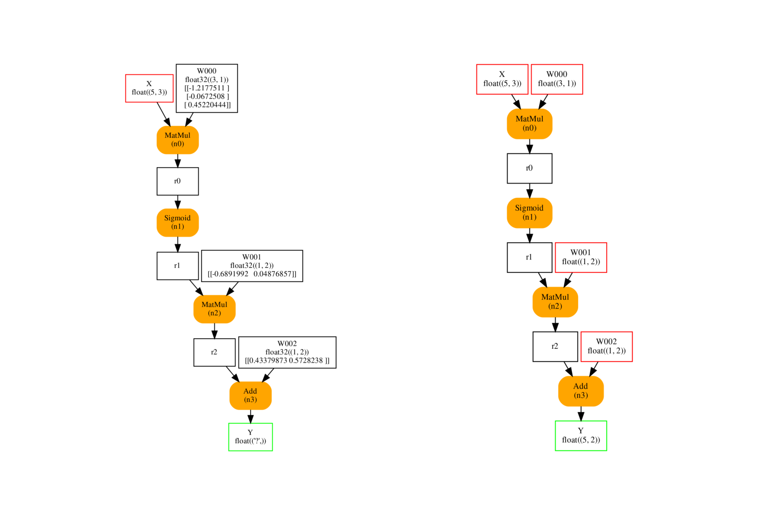
It produces the following inference graphs. The left one is the original one. The model on the left is the same except initializer are also inputs. If the input is missing, the initializer is considered as a default value.

fix, ax = plt.subplots(1, 2, figsize=(15, 10))
plot_onnx(onx, ax=ax[0])
plot_onnx(cls._optimized_pre_grad_model, ax=ax[1])

Out:

<AxesSubplot:>

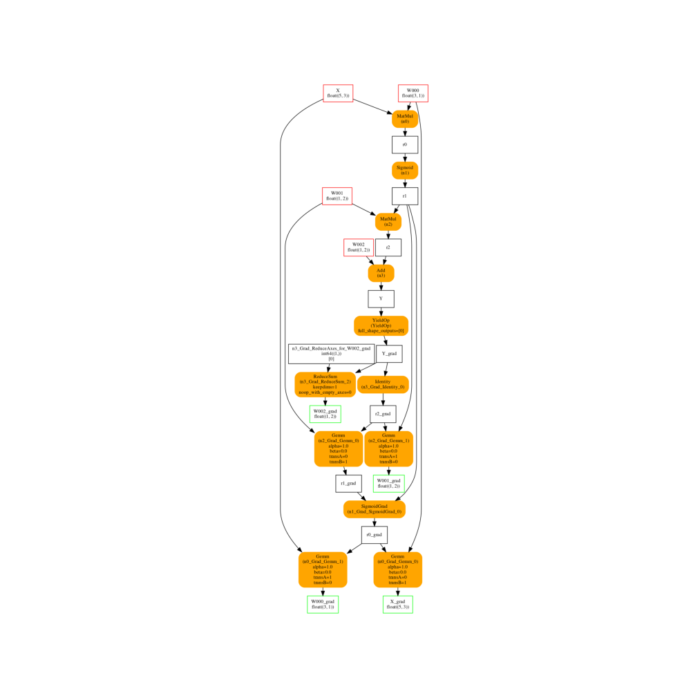
And the gradient graph. It has the same inputs the previous graph on the right and has an output for every trained parameter.

fix, ax = plt.subplots(1, 1, figsize=(10, 10))
plot_onnx(cls._trained_onnx, ax=ax)

Out:

<AxesSubplot:>

Training

We consider a simple example based on torch documentation (Learning Pytorch with Example or 110 - First percepton with pytorch).

def train_cls(cls, device, x, y, weights, n_iter=20, learning_rate=1e-2):
    x = from_numpy(x, requires_grad=True, device=device)
    y = from_numpy(y, requires_grad=True, device=device)

    weights_tch = [(w[0], from_numpy(w[1], requires_grad=True, device=device))
                   for w in weights]
    weights_values = [w[1] for w in weights_tch]

    all_losses = []
    for t in tqdm(range(n_iter)):
        # forward - backward
        y_pred = cls.apply(x, *weights_values)
        loss = (y_pred - y).pow(2).sum()
        loss.backward()

        # update weights
        with torch.no_grad():
            for name, w in weights_tch:
                w -= w.grad * learning_rate
                w.grad.zero_()

        all_losses.append((t, float(loss.cpu().detach().numpy())))
    return all_losses, weights_tch


device_name = "cuda:0" if torch.cuda.is_available() else "cpu"
device = torch.device(device_name)
print("device:", device)

x = numpy.random.randn(N, d_in).astype(numpy.float32)
y = numpy.random.randn(N, d_out).astype(numpy.float32)

train_losses, final_weights = train_cls(cls, device, x, y, weights)
train_losses = numpy.array(train_losses)
pprint.pprint(final_weights)

Out:

device: cpu

  0%|          | 0/20 [00:00<?, ?it/s]
100%|##########| 20/20 [00:00<00:00, 464.60it/s]
[('W000',
  tensor([[-1.2463],
        [-0.0078],
        [ 0.4170]], requires_grad=True)),
 ('W001', tensor([[-0.9162, -0.2614]], requires_grad=True)),
 ('W002', tensor([[0.2260, 0.2306]], requires_grad=True))]

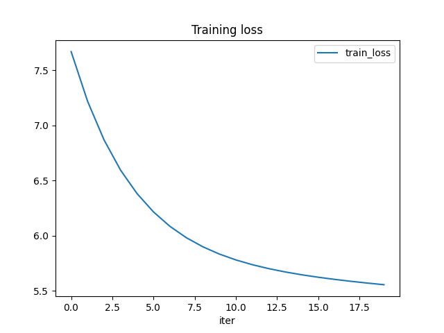
The training loss is decreasing. The function seems to be learning something.

df = DataFrame(data=train_losses, columns=['iter', 'train_loss'])
df.plot(x="iter", y="train_loss", title="Training loss")


# plt.show()

Out:

<AxesSubplot:title={'center':'Training loss'}, xlabel='iter'>

previous

Training

next

Pytorch and onnxruntime