p-values#
Links: notebook, html, PDF, python, slides, GitHub
Compute p-values and heavy tails estimators.
from jyquickhelper import add_notebook_menu
add_notebook_menu()
%matplotlib inline
p-value table#
from scipy.stats import norm
import pandas
from pandas import DataFrame
import numpy


def pvalue(p, q, N):
    theta   = abs(p-q)
    var     = p*(1-p)
    bn      = (2*N)**0.5 * theta / var**0.5
    ret     = (1 - norm.cdf(bn))*2
    return ret

def pvalue_N(p, q, alpha):
    theta   = abs(p-q)
    var     = p*(1-p)
    rev     = abs(norm.ppf (alpha/2))
    N       = 2 * (rev * var**0.5 / theta)** 2
    return int(N+1)

def alphatable(ps, dps, alpha):
    values = []
    for p in ps :
        row=[]
        for dp in dps :
            q = p+dp
            r = pvalue_N(p,q,alpha) if 1 >= q >= 0 else numpy.nan
            row.append (r)
        values.append (row)
    return values

def dataframe(ps,dps,table):
    columns = dps
    df = pandas.DataFrame(data=table, index=ps)
    df.columns = dps
    return df


print ("norm.ppf(0.025)",norm.ppf (0.025)) # -1.9599639845400545
ps  = [0.001, 0.002] + [ 0.05*i for i in range (1,20) ]
dps = [ -0.2, -0.1,  -0.02, -0.01, -0.002, -0.001,
         0.2,  0.1,   0.02,  0.01,  0.002,  0.001, ]
dps.sort()
t = alphatable(ps, dps, 0.05)
dataframe (ps, dps, t)
norm.ppf(0.025) -1.9599639845400545
| -0.200 | -0.100 | -0.020 | -0.010 | -0.002 | -0.001 | 0.001 | 0.002 | 0.010 | 0.020 | 0.100 | 0.200 | |
|---|---|---|---|---|---|---|---|---|---|---|---|---|
| 0.001 | NaN | NaN | NaN | NaN | NaN | 7676 | 7676 | 1919 | 77 | 20 | 1.0 | 1.0 |
| 0.002 | NaN | NaN | NaN | NaN | 3834.0 | 15336 | 15336 | 3834 | 154 | 39 | 2.0 | 1.0 |
| 0.050 | NaN | NaN | 913.0 | 3650.0 | 91235.0 | 364939 | 364939 | 91235 | 3650 | 913 | 37.0 | 10.0 |
| 0.100 | NaN | 70.0 | 1729.0 | 6915.0 | 172866.0 | 691463 | 691463 | 172866 | 6915 | 1729 | 70.0 | 18.0 |
| 0.150 | NaN | 98.0 | 2449.0 | 9796.0 | 244893.0 | 979572 | 979572 | 244893 | 9796 | 2449 | 98.0 | 25.0 |
| 0.200 | 31.0 | 123.0 | 3074.0 | 12293.0 | 307317.0 | 1229267 | 1229267 | 307317 | 12293 | 3074 | 123.0 | 31.0 |
| 0.250 | 37.0 | 145.0 | 3602.0 | 14406.0 | 360137.0 | 1440548 | 1440548 | 360137 | 14406 | 3602 | 145.0 | 37.0 |
| 0.300 | 41.0 | 162.0 | 4034.0 | 16135.0 | 403354.0 | 1613413 | 1613413 | 403354 | 16135 | 4034 | 162.0 | 41.0 |
| 0.350 | 44.0 | 175.0 | 4370.0 | 17479.0 | 436966.0 | 1747864 | 1747864 | 436966 | 17479 | 4370 | 175.0 | 44.0 |
| 0.400 | 47.0 | 185.0 | 4610.0 | 18440.0 | 460976.0 | 1843901 | 1843901 | 460976 | 18440 | 4610 | 185.0 | 47.0 |
| 0.450 | 48.0 | 191.0 | 4754.0 | 19016.0 | 475381.0 | 1901523 | 1901523 | 475381 | 19016 | 4754 | 191.0 | 48.0 |
| 0.500 | 49.0 | 193.0 | 4802.0 | 19208.0 | 480183.0 | 1920730 | 1920730 | 480183 | 19208 | 4802 | 193.0 | 49.0 |
| 0.550 | 48.0 | 191.0 | 4754.0 | 19016.0 | 475381.0 | 1901523 | 1901523 | 475381 | 19016 | 4754 | 191.0 | 48.0 |
| 0.600 | 47.0 | 185.0 | 4610.0 | 18440.0 | 460976.0 | 1843901 | 1843901 | 460976 | 18440 | 4610 | 185.0 | 47.0 |
| 0.650 | 44.0 | 175.0 | 4370.0 | 17479.0 | 436966.0 | 1747864 | 1747864 | 436966 | 17479 | 4370 | 175.0 | 44.0 |
| 0.700 | 41.0 | 162.0 | 4034.0 | 16135.0 | 403354.0 | 1613413 | 1613413 | 403354 | 16135 | 4034 | 162.0 | 41.0 |
| 0.750 | 37.0 | 145.0 | 3602.0 | 14406.0 | 360137.0 | 1440548 | 1440548 | 360137 | 14406 | 3602 | 145.0 | 37.0 |
| 0.800 | 31.0 | 123.0 | 3074.0 | 12293.0 | 307317.0 | 1229267 | 1229267 | 307317 | 12293 | 3074 | 123.0 | 31.0 |
| 0.850 | 25.0 | 98.0 | 2449.0 | 9796.0 | 244893.0 | 979572 | 979572 | 244893 | 9796 | 2449 | 98.0 | NaN |
| 0.900 | 18.0 | 70.0 | 1729.0 | 6915.0 | 172866.0 | 691463 | 691463 | 172866 | 6915 | 1729 | 70.0 | NaN |
| 0.950 | 10.0 | 37.0 | 913.0 | 3650.0 | 91235.0 | 364939 | 364939 | 91235 | 3650 | 913 | NaN | NaN |
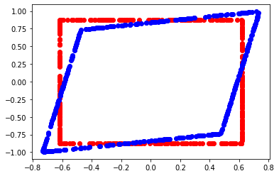
p-values in 2D#
import numpy, matplotlib, random, math
import matplotlib.pyplot as pylab
def matrix_square_root(sigma) :
eigen, vect = numpy.linalg.eig(sigma)
dim = len(sigma)
res = numpy.identity(dim)
for i in range(0,dim) :
res[i,i] = eigen[i]**0.5
return vect * res * vect.transpose()
def chi2_level (alpha = 0.95) :
N = 1000
x = [ random.gauss(0,1) for _ in range(0,N) ]
y = [ random.gauss(0,1) for _ in range(0,N) ]
r = map ( lambda c : (c[0]**2+c[1]**2)**0.5, zip(x,y))
r = list(r)
r.sort()
res = r [ int (alpha * N) ]
return res
def square_figure(mat, a) :
x = [ ]
y = [ ]
for i in range (0,100) :
x.append( a * mat[0][0]**0.5 )
y.append( (random.random ()-0.5) * a * mat[1][1]**0.5*2 )
x.append( -a * mat[0][0]**0.5 )
y.append( (random.random ()-0.5) * a * mat[1][1]**0.5*2 )
y.append( a * mat[1][1]**0.5 )
x.append( (random.random ()-0.5) * a * mat[0][0]**0.5*2 )
y.append( -a * mat[1][1]**0.5 )
x.append( (random.random ()-0.5) * a * mat[0][0]**0.5*2 )
pylab.plot(x,y, 'ro')
x = [ ]
y = [ ]
for i in range (0,100) :
x.append( a )
y.append( (random.random ()-0.5) * a*2 )
x.append( -a )
y.append( (random.random ()-0.5) * a*2 )
y.append( a )
x.append( (random.random ()-0.5) * a*2 )
y.append( -a )
x.append( (random.random ()-0.5) * a*2 )
xs,ys = [],[]
for a,b in zip (x,y) :
ar = numpy.matrix( [ [a], [b] ] ).transpose()
we = ar * root
xs.append( we [0,0] )
ys.append( we [0,1] )
pylab.plot(xs,ys, 'bo')
pylab.show()
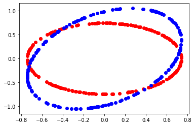
def circle_figure (mat, a) :
x = [ ]
y = [ ]
for i in range (0,200) :
z = random.random() * math.pi * 2
i = a * mat[0][0]**0.5 * math.cos(z)
j = a * mat[0][0]**0.5 * math.sin(z)
x.append ( i )
y.append ( j )
pylab.plot(x,y, 'ro')
x = [ ]
y = [ ]
for i in range (0,200) :
z = random.random() * math.pi * 2
i = a * math.cos(z)
j = a * math.sin(z)
x.append ( i )
y.append ( j )
xs,ys = [],[]
for a,b in zip (x,y) :
ar = numpy.matrix( [ [a], [b] ] ).transpose()
we = ar * root
xs.append( we [0,0] )
ys.append( we [0,1] )
pylab.plot(xs,ys, 'bo')
pylab.show()
level = chi2_level ()
mat = [ [0.1, 0.05], [0.05, 0.2] ]
npmat = numpy.matrix(mat)
root = matrix_square_root (npmat)
square_figure (mat, 1.96)
circle_figure (mat, level)
p-value ratio#
import random, math

def densite_gauss (mu, sigma, x) :
    e = -(x - mu)**2 / (sigma**2 * 2)
    d = 1. / ((2*math.pi)**0.5 * sigma)
    return d * math.exp (e)

def simulation_vector (N, mu, sigma) :
    return [ random.gauss(mu,sigma) for n in range(N) ]

def ratio (vector, x, fdensite) :
    under = 0
    above = 0
    fx    = fdensite(x)
    for u in vector:
        f = fdensite (u)
        if f >= fx:
            above += 1
        else:
            under += 1
    return float(above) / float (above + under)

x     = 1.96
N     = 10000
mu    = 0
sigma = 1

v = simulation_vector(N, mu, sigma)
g = ratio(v, x, lambda y: densite_gauss (mu, sigma, y) )
print (g)
0.9487
p-values and EM#
See Applying the EM Algorithm: Binomial Mixtures.
from scipy.stats import norm
import random, math


def average_std_deviation(sample):
    mean = 0.
    var  = 0.
    for x in sample:
        mean += x
        var += x*x
    mean /= len(sample)
    var /= len(sample)
    var -= mean*mean
    return mean,var ** 0.5

def bootsample(sample):
    n = len(sample)-1
    return [ sample[ random.randint(0,n) ] for _ in sample ]

def bootstrap_difference(sampleX, sampleY, draws=2000, confidence=0.05):
    diff = [ ]
    for n in range (0,draws) :
        if n % 1000 == 0:
            print(n)
        sx = bootsample(sampleX)
        sy = bootsample(sampleY)
        px = sum(sx) * 1.0/ len(sx)
        py = sum(sy) * 1.0/ len(sy)
        diff.append (px-py)
    diff.sort()
    n = int(len(diff) * confidence / 2)
    av = sum(diff) / len(diff)
    return av, diff [n], diff [len(diff)-n]

# generation of a sample

def generate_obs(p):
    x = random.random()
    if x <= p : return 1
    else : return 0

def generate_n_obs(p, n):
    return [ generate_obs(p) for i in range (0,n) ]

# std deviation

def diff_std_deviation(px, py):
    s = px*(1-px) + py*(1-py)
    return px, py, s**0.5

def pvalue(diff, std, N):
    theta = abs(diff)
    bn = (2*N)**0.5 * theta / std
    pv = (1 - norm.cdf(bn))*2
    return pv

def omega_i (X, pi, p, q) :
    np = p * pi     if X == 1 else (1-p)*pi
    nq = q * (1-pi) if X == 1 else (1-q)*(1-pi)
    return np / (np + nq)

def likelihood (X, pi, p, q) :
    np = p * pi     if X == 1 else (1-p)*pi
    nq = q * (1-pi) if X == 1 else (1-q)*(1-pi)
    return math.log(np) + math.log(nq)

def algoEM (sample):
    p   = random.random()
    q   = random.random()
    pi  = random.random()
    iter   = 0
    while iter < 10 :
        lk = sum ( [ likelihood (x, pi, p, q) for x in sample ] )
        wi  = [ omega_i (x, pi, p, q) for x in sample ]
        sw  = sum(wi)
        pin = sum(wi) / len(wi)
        pn  = sum([ x * w     for x,w in zip (sample,wi) ]) / sw
        qn  = sum([ x * (1-w) for x,w in zip (sample,wi) ]) / (len(wi) - sw)

        pi,p,q = pin,pn,qn
        iter += 1

    lk = sum ( [ likelihood (x, pi, p, q) for x in sample ] )
    return pi,p,q, lk


# mix
p,q   = 0.20, 0.80
pi    = 0.7
N     = 1000
na    = int(N * pi)
nb    = N - na

print("------- sample")
sampleX = generate_n_obs(p, na) + generate_n_obs (q, nb)
random.shuffle(sampleX)
print("ave", p * pi + q*(1-pi))
print("mea", sum(sampleX)*1./len(sampleX))

lk = sum ( [ likelihood (x, pi, p, q) for x in sampleX ] )
print ("min lk", lk, sum (sampleX)*1. / len(sampleX))
res = []
for k in range (0, 10) :
    r = algoEM (sampleX)
    res.append ( (r[-1], r) )
res.sort ()

rows = []
for r in res:
    pi,p,q,lk = r[1]
    rows.append( [p * pi + q*(1-pi)] + list(r[1]))

df = pandas.DataFrame(data=rows)
df.columns = ["average", "pi", "p", "q", "likelihood"]
df
------- sample
ave 0.38
mea 0.373
min lk -3393.2292120130046 0.373
| average | pi | p | q | likelihood | |
|---|---|---|---|---|---|
| 0 | 0.373 | 0.000324 | 0.341877 | 0.373010 | -9358.705695 |
| 1 | 0.373 | 0.863747 | 0.284788 | 0.932204 | -4531.967709 |
| 2 | 0.373 | 0.936083 | 0.346101 | 0.766941 | -4490.512057 |
| 3 | 0.373 | 0.123023 | 0.290964 | 0.384508 | -3563.557269 |
| 4 | 0.373 | 0.538835 | 0.053584 | 0.746213 | -3487.438442 |
| 5 | 0.373 | 0.346351 | 0.057880 | 0.539974 | -3302.391944 |
| 6 | 0.373 | 0.797540 | 0.376491 | 0.359248 | -3144.938682 |
| 7 | 0.373 | 0.392520 | 0.592563 | 0.231131 | -2902.915478 |
| 8 | 0.373 | 0.390241 | 0.459488 | 0.317648 | -2778.903072 |
| 9 | 0.373 | 0.609127 | 0.338062 | 0.427447 | -2764.987703 |
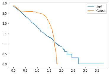
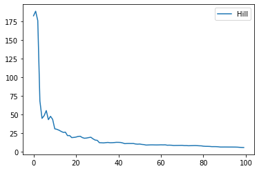
p-value and heavy tail#
from scipy.stats import norm, zipf
import sys


def generate_n_obs_zipf (tail_index, n) :
    return list(zipf.rvs(tail_index, size=n))

def hill_estimator (sample) :
    sample = list(sample)
    sample.sort(reverse=True)
    end = len(sample)/10
    end = min(end,100)
    s = 0.
    res = []
    for k in range (0,end) :
        s += math.log(sample[k])
        h = (s - (k+1)*math.log(sample[k+1]))/(k+1)
        h = 1./h
        res.append( [k, h] )
    return res

# mix
tail_index  = 1.05
N           = 10000

sample = generate_n_obs_zipf(tail_index, N)
sample[:5]
[357621, 148, 18, 1812876449, 36150]
import pandas
def graph_XY(curves, xlabel=None, ylabel=None, marker=True,
link_point=False, title=None, format_date="%Y-%m-%d",
legend_loc=0, figsize=None, ax=None):
if ax is None:
import matplotlib.pyplot as plt # pylint: disable=C0415
fig, ax = plt.subplots(1, 1, figsize=figsize)
smarker = {(True, True): 'o-', (True, False): 'o', (False, True): '-',
# (False, False) :''
}[marker, link_point]
has_date = False
for xf, yf, label in curves:
ax.plot(xf, yf, smarker, label=label)
ax.legend(loc=legend_loc)
return ax
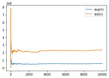
def draw_variance(sample) :
avg = 0.
std = 0.
n = 0.
w = 1.
add = []
for i,x in enumerate(sample) :
x = float (x)
avg += x * w
std += x*x * w
n += w
val = (std/n - (avg/n)**2)**0.5
add.append ( [ i, avg/n, val] )
print(add[-1])
table = pandas.DataFrame(add, columns=["index", "avg(n)", "std(n)"])
return graph_XY([
[table['index'], table["avg(n)"], "avg(n)"],
[table['index'], table["std(n)"], "std(n)"],
], marker=False, link_point=True)
draw_variance(sample);
[9999, 55186871.0339, 233342554.46156308]
def draw_hill_estimator (sample) :
    res = hill_estimator(sample)
    table = DataFrame(res, columns=["d", "hill"])
    return graph_XY(
        [[table['d'], table['hill'], "Hill"],],
        marker=False, link_point=True)

draw_hill_estimator(sample);
def draw_heavy_tail (sample) :
    table   = DataFrame([[_] for _ in sample ], columns=["obs"])
    std = 1

    normal = norm.rvs(size = len(sample))
    normal = [ x*std  for x in normal ]
    nortbl = DataFrame([ [_] for _ in normal ], columns=["obs"])
    nortbl["iobs"] = (nortbl['obs'] * 10).astype(numpy.int64)

    histon = nortbl[["iobs", "obs"]].groupby('iobs', as_index=False).count()
    histon.columns = ['iobs', 'nb']
    histon = histon.sort_values("nb", ascending=False).reset_index(drop=True)

    table["one"] = 1
    histo = table.groupby('obs', as_index=False).count()
    histo.columns = ['obs', 'nb']
    histo = histo.sort_values('nb', ascending=False).reset_index(drop=True)
    histo.reset_index(drop=True, inplace=True)
    histo["index"] = histo.index + 1

    vec  = list(histon["nb"])
    vec += [0,] * len(histo)
    histo['nb_normal'] = vec[:len(histo)]

    histo["log(index)"] = numpy.log(histo["index"]) / numpy.log(10)
    histo["log(nb)"] = numpy.log(histo["nb"]) / numpy.log(10)
    histo["log(nb_normal)"] = numpy.log(histo["nb_normal"]) / numpy.log(10)
    return graph_XY ([
            [histo["log(index)"], histo["log(nb)"], "Zipf"],
            [histo["log(index)"], histo["log(nb_normal)"], "Gauss"], ],
                     marker=False, link_point=True)

draw_heavy_tail(sample);
c:python372_x64libsite-packagespandascoreseries.py:679: RuntimeWarning: divide by zero encountered in log
  result = getattr(ufunc, method)(*inputs, **kwargs)