LogisticRegression and Clustering

Links: notebook, html, PDF, python, slides, GitHub

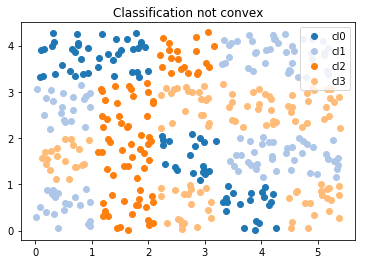
A logistic regression implements a convex partition of the features spaces. A clustering algorithm applied before the trainer modifies the feature space in way the partition is not necessarily convex in the initial features. Let’s see how.

from jyquickhelper import add_notebook_menu
add_notebook_menu()

%matplotlib inline

A dummy datasets and not convex

import numpy
import numpy.random
Xs = []
Ys = []
n = 20
for i in range(0, 5):
    for j in range(0, 4):
        x1 = numpy.random.rand(n) + i*1.1
        x2 = numpy.random.rand(n) + j*1.1
        Xs.append(numpy.vstack([x1,x2]).T)
        cl = numpy.random.randint(0, 4)
        Ys.extend([cl for i in range(n)])
X = numpy.vstack(Xs)
Y = numpy.array(Ys)
X.shape, Y.shape, set(Y)

((400, 2), (400,), {0, 1, 2, 3})

import matplotlib.pyplot as plt
fig, ax = plt.subplots(1, 1, figsize=(6,4))
for i in set(Y):
    ax.plot(X[Y==i,0], X[Y==i,1], 'o', label="cl%d"%i, color=plt.cm.tab20.colors[i])
ax.legend()
ax.set_title("Classification not convex");

One function to plot classification in 2D

import matplotlib.pyplot as plt

def draw_border(clr, X, y, fct=None, incx=1, incy=1, figsize=None, border=True, clusters=None, ax=None):

    # see https://sashat.me/2017/01/11/list-of-20-simple-distinct-colors/
    # https://matplotlib.org/examples/color/colormaps_reference.html
    _unused_ = ["Red", "Green", "Yellow", "Blue", "Orange", "Purple", "Cyan",
              "Magenta", "Lime", "Pink", "Teal", "Lavender", "Brown", "Beige",
              "Maroon", "Mint", "Olive", "Coral", "Navy", "Grey", "White", "Black"]

    h = .02  # step size in the mesh
    # Plot the decision boundary. For that, we will assign a color to each
    # point in the mesh [x_min, x_max]x[y_min, y_max].
    x_min, x_max = X[:, 0].min() - incx, X[:, 0].max() + incx
    y_min, y_max = X[:, 1].min() - incy, X[:, 1].max() + incy
    xx, yy = numpy.meshgrid(numpy.arange(x_min, x_max, h), numpy.arange(y_min, y_max, h))
    if fct is None:
        Z = clr.predict(numpy.c_[xx.ravel(), yy.ravel()])
    else:
        Z = fct(clr, numpy.c_[xx.ravel(), yy.ravel()])

    # Put the result into a color plot
    cmap = plt.cm.tab20
    Z = Z.reshape(xx.shape)
    if ax is None:
        fig, ax = plt.subplots(1, 1, figsize=figsize or (4, 3))
    ax.pcolormesh(xx, yy, Z, cmap=cmap)

    # Plot also the training points
    ax.scatter(X[:, 0], X[:, 1], c=y, edgecolors='k', cmap=cmap)
    ax.set_xlabel('Sepal length')
    ax.set_ylabel('Sepal width')

    ax.set_xlim(xx.min(), xx.max())
    ax.set_ylim(yy.min(), yy.max())

    # Plot clusters
    if clusters is not None:
        mat = []
        ym = []
        for k, v in clusters.items():
            mat.append(v.cluster_centers_)
            ym.extend(k for i in range(v.cluster_centers_.shape[0]))
        cx = numpy.vstack(mat)
        ym = numpy.array(ym)
        ax.scatter(cx[:, 0], cx[:, 1], c=ym, edgecolors='y', cmap=cmap, s=300)
    return ax

Logistic Regression

from sklearn.linear_model import LogisticRegression
clr = LogisticRegression(solver='lbfgs', multi_class='multinomial')
clr.fit(X, Y)

LogisticRegression(C=1.0, class_weight=None, dual=False, fit_intercept=True,
          intercept_scaling=1, max_iter=100, multi_class='multinomial',
          n_jobs=None, penalty='l2', random_state=None, solver='lbfgs',
          tol=0.0001, verbose=0, warm_start=False)

ax = draw_border(clr, X, Y, incx=1, incy=1, figsize=(6,4), border=False)
ax.set_title("Logistic Regression");

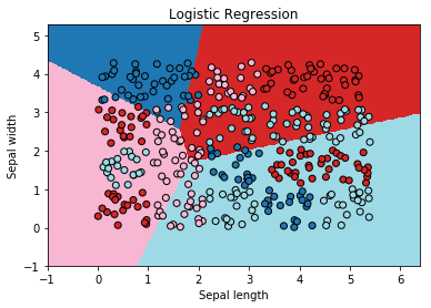
Not quite close!

Logistic Regression and k-means

from mlinsights.mlmodel import ClassifierAfterKMeans
clk = ClassifierAfterKMeans(e_solver='lbfgs', e_multi_class='multinomial')
clk.fit(X, Y)

c:python370_x64libsite-packagessklearnlinear_modellogistic.py:757: ConvergenceWarning: lbfgs failed to converge. Increase the number of iterations.
  "of iterations.", ConvergenceWarning)

ClassifierAfterKMeans(c_algorithm='auto', c_copy_x=True, c_init='k-means++',
           c_max_iter=300, c_n_clusters=2, c_n_init=10, c_n_jobs=None,
           c_precompute_distances='auto', c_random_state=None,
           c_tol=0.0001, c_verbose=0, e_C=1.0, e_class_weight=None,
           e_dual=False, e_fit_intercept=True, e_intercept_scaling=1,
           e_max_iter=100, e_multi_class='multinomial', e_n_jobs=None,
           e_penalty='l2', e_random_state=None, e_solver='lbfgs',
           e_tol=0.0001, e_verbose=0, e_warm_start=False)

The centers of the first k-means:

clk.clus_[0].cluster_centers_

array([[3.26205371, 1.08211905],
       [1.06113799, 3.78383125]])

ax = draw_border(clk, X, Y, incx=1, incy=1, figsize=(6,4), border=False, clusters=clk.clus_)
ax.set_title("Logistic Regression and K-Means - 2 clusters per class");

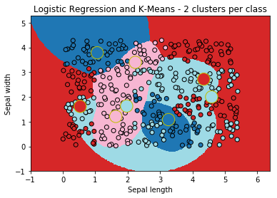
The big cricles are the centers of the k-means fitted for each class. It look better!

Variation

dt = []
for cl in range(1, 6):
    clk = ClassifierAfterKMeans(c_n_clusters=cl, e_solver='lbfgs',
                                e_multi_class='multinomial', e_max_iter=700)
    clk.fit(X, Y)
    sc = clk.score(X,Y)
    dt.append(dict(score=sc, nb_clusters=cl))
import pandas
pandas.DataFrame(dt)

	nb_clusters	score
0	1	0.4475
1	2	0.6600
2	3	0.7475
3	4	0.8400
4	5	0.9200

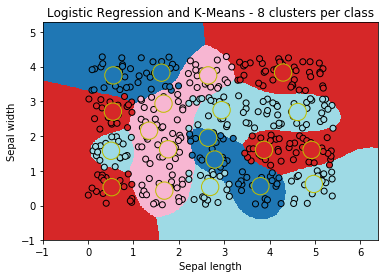
ax = draw_border(clk, X, Y, incx=1, incy=1, figsize=(6,4), border=False, clusters=clk.clus_)
ax.set_title("Logistic Regression and K-Means - 8 clusters per class");

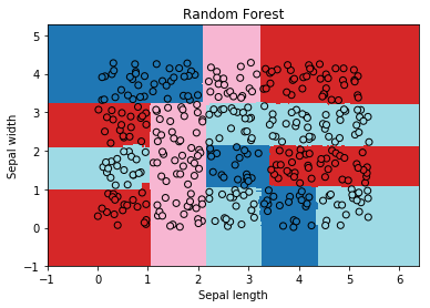
Random Forest

The random forest works without any clustering as expected.

from sklearn.ensemble import RandomForestClassifier
rf = RandomForestClassifier(n_estimators=20)
rf.fit(X, Y)

RandomForestClassifier(bootstrap=True, class_weight=None, criterion='gini',
            max_depth=None, max_features='auto', max_leaf_nodes=None,
            min_impurity_decrease=0.0, min_impurity_split=None,
            min_samples_leaf=1, min_samples_split=2,
            min_weight_fraction_leaf=0.0, n_estimators=20, n_jobs=None,
            oob_score=False, random_state=None, verbose=0,
            warm_start=False)

ax = draw_border(rf, X, Y, incx=1, incy=1, figsize=(6,4), border=False)
ax.set_title("Random Forest");