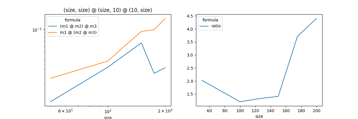
Associativity and matrix multiplication

The matrix multiplication m1 @ m2 @ m3 can be done in two different ways: (m1 @ m2) @ m3 or m1 @ (m2 @ m3). Are these two orders equivalent or is there a better order?

import pprint
import numpy
import matplotlib.pyplot as plt
from pandas import DataFrame
from tqdm import tqdm
from td3a_cpp.tools import measure_time

First try

m1 = numpy.random.rand(100, 100)
m2 = numpy.random.rand(100, 10)
m3 = numpy.random.rand(10, 100)

m = m1 @ m2 @ m3

print(m.shape)

mm1 = (m1 @ m2) @ m3
mm2 = m1 @ (m2 @ m3)

print(mm1.shape, mm2.shape)

t1 = measure_time(lambda: (m1 @ m2) @ m3, context={}, number=100, repeat=100)
pprint.pprint(t1)

t2 = measure_time(lambda: m1 @ (m2 @ m3), context={}, number=100, repeat=100)
pprint.pprint(t2)

(100, 100)
(100, 100) (100, 100)
{'average': 0.0003212100610136986,
 'context_size': 232,
 'deviation': 3.68551974980911e-07,
 'max_exec': 0.0003237356524914503,
 'min_exec': 0.0003209231933578849,
 'number': 100,
 'repeat': 100}
{'average': 0.0003866767174098639,
 'context_size': 232,
 'deviation': 1.337162285443633e-06,
 'max_exec': 0.0003964086202904582,
 'min_exec': 0.0003854487417265773,
 'number': 100,
 'repeat': 100}

With different sizes

obs = []
for i in tqdm([50, 100, 125, 150, 175, 200]):

    m1 = numpy.random.rand(i, i)
    m2 = numpy.random.rand(i, 10)
    m3 = numpy.random.rand(10, i)

    t1 = measure_time(lambda: (m1 @ m2) @ m3,
                      context={}, number=100, repeat=100)
    t1['formula'] = "(m1 @ m2) @ m3"
    t1['size'] = i
    obs.append(t1)
    t2 = measure_time(lambda: m1 @ (m2 @ m3),
                      context={}, number=100, repeat=100)
    t2['formula'] = "m1 @ (m2 @ m3)"
    t2['size'] = i
    obs.append(t2)

df = DataFrame(obs)
piv = df.pivot(index="size", columns="formula", values="average")
piv

  0%|          | 0/6 [00:00<?, ?it/s]
 17%|#6        | 1/6 [00:03<00:17,  3.44s/it]
 33%|###3      | 2/6 [00:10<00:22,  5.58s/it]
 50%|#####     | 3/6 [00:21<00:24,  8.11s/it]
 67%|######6   | 4/6 [00:37<00:22, 11.27s/it]
 83%|########3 | 5/6 [00:50<00:11, 11.73s/it]
100%|##########| 6/6 [01:07<00:00, 13.55s/it]
100%|##########| 6/6 [01:07<00:00, 11.23s/it]

formula	(m1 @ m2) @ m3	m1 @ (m2 @ m3)
size
50	0.000114	0.000230
100	0.000321	0.000386
125	0.000479	0.000633
150	0.000668	0.000941
175	0.000267	0.000988
200	0.000316	0.001391

Graph

fig, ax = plt.subplots(1, 2, figsize=(12, 4))
piv.plot(logx=True, logy=True, ax=ax[0],
         title=f"{m1.shape!r} @ {m2.shape!r} @ "
               f"{m3.shape!r}".replace("200", "size"))
piv["ratio"] = piv["m1 @ (m2 @ m3)"] / piv["(m1 @ m2) @ m3"]
piv[['ratio']].plot(ax=ax[1])

plt.show()