Compares dot implementations (numpy, python, blas)

numpy has a very fast implementation of the dot product. It is difficult to be better and very easy to be slower. This example looks into a couple of slower implementations.

Compared implementations:

• pydot

• cblas_ddot

import pprint
import numpy
import matplotlib.pyplot as plt
from pandas import DataFrame, concat
from td3a_cpp.tutorial import pydot, cblas_ddot
from td3a_cpp.tools import measure_time_dim

python dot: pydot

The first function pydot uses python to implement the dot product.

ctxs = [dict(va=numpy.random.randn(n).astype(numpy.float64),
             vb=numpy.random.randn(n).astype(numpy.float64),
             pydot=pydot,
             x_name=n)
        for n in range(10, 1000, 100)]

res_pydot = list(measure_time_dim('pydot(va, vb)', ctxs, verbose=1))

pprint.pprint(res_pydot[:2])

  0%|          | 0/10 [00:00<?, ?it/s]
 30%|###       | 3/10 [00:00<00:00, 18.30it/s]
 50%|#####     | 5/10 [00:00<00:00,  9.46it/s]
 70%|#######   | 7/10 [00:00<00:00,  6.16it/s]
 80%|########  | 8/10 [00:01<00:00,  5.11it/s]
 90%|######### | 9/10 [00:01<00:00,  4.32it/s]
100%|##########| 10/10 [00:02<00:00,  3.68it/s]
100%|##########| 10/10 [00:02<00:00,  4.98it/s]
[{'average': 2.4982207454741003e-05,
  'context_size': 232,
  'deviation': 4.265833773511768e-07,
  'max_exec': 2.5938916951417924e-05,
  'min_exec': 2.463754266500473e-05,
  'number': 50,
  'repeat': 10,
  'x_name': 10},
 {'average': 0.00010771532170474529,
  'context_size': 232,
  'deviation': 4.2879408576822083e-07,
  'max_exec': 0.00010854371823370456,
  'min_exec': 0.000107117323204875,
  'number': 50,
  'repeat': 10,
  'x_name': 110}]

numpy dot

ctxs = [dict(va=numpy.random.randn(n).astype(numpy.float64),
             vb=numpy.random.randn(n).astype(numpy.float64),
             dot=numpy.dot,
             x_name=n)
        for n in range(10, 50000, 100)]

res_dot = list(measure_time_dim('dot(va, vb)', ctxs, verbose=1))

pprint.pprint(res_dot[:2])

  0%|          | 0/500 [00:00<?, ?it/s]
  4%|3         | 18/500 [00:00<00:02, 177.61it/s]
  7%|7         | 36/500 [00:00<00:02, 156.16it/s]
 10%|#         | 52/500 [00:00<00:03, 140.54it/s]
 13%|#3        | 67/500 [00:00<00:03, 127.80it/s]
 16%|#6        | 80/500 [00:00<00:03, 117.82it/s]
 18%|#8        | 92/500 [00:00<00:03, 109.21it/s]
 21%|##        | 104/500 [00:00<00:03, 103.48it/s]
 23%|##3       | 115/500 [00:00<00:03, 102.50it/s]
 25%|##5       | 126/500 [00:01<00:03, 101.31it/s]
 27%|##7       | 137/500 [00:01<00:03, 100.02it/s]
 30%|##9       | 148/500 [00:01<00:03, 98.72it/s]
 32%|###1      | 158/500 [00:01<00:03, 97.45it/s]
 34%|###3      | 168/500 [00:01<00:03, 96.43it/s]
 36%|###5      | 178/500 [00:01<00:03, 95.29it/s]
 38%|###7      | 188/500 [00:01<00:03, 94.51it/s]
 40%|###9      | 198/500 [00:01<00:03, 93.57it/s]
 42%|####1     | 208/500 [00:01<00:03, 92.69it/s]
 44%|####3     | 218/500 [00:02<00:03, 91.85it/s]
 46%|####5     | 228/500 [00:02<00:02, 91.01it/s]
 48%|####7     | 238/500 [00:02<00:02, 90.24it/s]
 50%|####9     | 248/500 [00:02<00:02, 89.50it/s]
 51%|#####1    | 257/500 [00:02<00:02, 88.67it/s]
 53%|#####3    | 266/500 [00:02<00:02, 87.97it/s]
 55%|#####5    | 275/500 [00:02<00:02, 87.28it/s]
 57%|#####6    | 284/500 [00:02<00:02, 86.58it/s]
 59%|#####8    | 293/500 [00:02<00:02, 85.90it/s]
 60%|######    | 302/500 [00:03<00:02, 85.22it/s]
 62%|######2   | 311/500 [00:03<00:02, 84.66it/s]
 64%|######4   | 320/500 [00:03<00:02, 84.13it/s]
 66%|######5   | 329/500 [00:03<00:02, 83.50it/s]
 68%|######7   | 338/500 [00:03<00:01, 82.86it/s]
 69%|######9   | 347/500 [00:03<00:01, 82.34it/s]
 71%|#######1  | 356/500 [00:03<00:01, 81.73it/s]
 73%|#######3  | 365/500 [00:03<00:01, 81.24it/s]
 75%|#######4  | 374/500 [00:03<00:01, 80.68it/s]
 77%|#######6  | 383/500 [00:04<00:01, 80.10it/s]
 78%|#######8  | 392/500 [00:04<00:01, 79.69it/s]
 80%|########  | 400/500 [00:04<00:01, 79.13it/s]
 82%|########1 | 408/500 [00:04<00:01, 78.72it/s]
 83%|########3 | 416/500 [00:04<00:01, 78.20it/s]
 85%|########4 | 424/500 [00:04<00:00, 77.67it/s]
 86%|########6 | 432/500 [00:04<00:00, 76.87it/s]
 88%|########8 | 440/500 [00:04<00:00, 76.24it/s]
 90%|########9 | 448/500 [00:04<00:00, 75.61it/s]
 91%|#########1| 456/500 [00:05<00:00, 75.30it/s]
 93%|#########2| 464/500 [00:05<00:00, 74.93it/s]
 94%|#########4| 472/500 [00:05<00:00, 74.54it/s]
 96%|#########6| 480/500 [00:05<00:00, 74.21it/s]
 98%|#########7| 488/500 [00:05<00:00, 73.95it/s]
 99%|#########9| 496/500 [00:05<00:00, 73.45it/s]
100%|##########| 500/500 [00:05<00:00, 88.94it/s]
[{'average': 8.04197695106268e-06,
  'context_size': 232,
  'deviation': 3.954607054646713e-07,
  'max_exec': 9.134504944086075e-06,
  'min_exec': 7.828520610928535e-06,
  'number': 50,
  'repeat': 10,
  'x_name': 10},
 {'average': 8.221659809350966e-06,
  'context_size': 232,
  'deviation': 1.974098308461028e-07,
  'max_exec': 8.763503283262253e-06,
  'min_exec': 8.071912452578544e-06,
  'number': 50,
  'repeat': 10,
  'x_name': 110}]

blas dot

numpy implementation uses BLAS. Let’s make a direct call to it.

for ctx in ctxs:
    ctx['ddot'] = cblas_ddot

res_ddot = list(measure_time_dim('ddot(va, vb)', ctxs, verbose=1))

pprint.pprint(res_ddot[:2])

  0%|          | 0/500 [00:00<?, ?it/s]
  3%|3         | 16/500 [00:00<00:03, 154.83it/s]
  6%|6         | 32/500 [00:00<00:03, 139.00it/s]
  9%|9         | 47/500 [00:00<00:03, 126.78it/s]
 12%|#2        | 60/500 [00:00<00:03, 117.33it/s]
 14%|#4        | 72/500 [00:00<00:03, 109.19it/s]
 17%|#6        | 83/500 [00:00<00:04, 102.13it/s]
 19%|#8        | 94/500 [00:00<00:04, 95.61it/s]
 21%|##        | 104/500 [00:01<00:04, 88.13it/s]
 23%|##2       | 113/500 [00:01<00:04, 84.43it/s]
 24%|##4       | 122/500 [00:01<00:04, 84.38it/s]
 26%|##6       | 131/500 [00:01<00:04, 85.79it/s]
 28%|##8       | 140/500 [00:01<00:04, 86.67it/s]
 30%|##9       | 149/500 [00:01<00:04, 87.09it/s]
 32%|###1      | 158/500 [00:01<00:03, 87.10it/s]
 33%|###3      | 167/500 [00:01<00:03, 87.02it/s]
 35%|###5      | 176/500 [00:01<00:03, 86.59it/s]
 37%|###7      | 185/500 [00:01<00:03, 86.12it/s]
 39%|###8      | 194/500 [00:02<00:03, 85.70it/s]
 41%|####      | 203/500 [00:02<00:03, 85.24it/s]
 42%|####2     | 212/500 [00:02<00:03, 84.48it/s]
 44%|####4     | 221/500 [00:02<00:03, 83.92it/s]
 46%|####6     | 230/500 [00:02<00:03, 83.33it/s]
 48%|####7     | 239/500 [00:02<00:03, 82.76it/s]
 50%|####9     | 248/500 [00:02<00:03, 82.22it/s]
 51%|#####1    | 257/500 [00:02<00:02, 81.59it/s]
 53%|#####3    | 266/500 [00:02<00:02, 81.01it/s]
 55%|#####5    | 275/500 [00:03<00:02, 80.46it/s]
 57%|#####6    | 284/500 [00:03<00:02, 79.89it/s]
 58%|#####8    | 292/500 [00:03<00:02, 79.42it/s]
 60%|######    | 300/500 [00:03<00:02, 78.91it/s]
 62%|######1   | 308/500 [00:03<00:02, 78.36it/s]
 63%|######3   | 316/500 [00:03<00:02, 77.97it/s]
 65%|######4   | 324/500 [00:03<00:02, 77.54it/s]
 66%|######6   | 332/500 [00:03<00:02, 77.03it/s]
 68%|######8   | 340/500 [00:03<00:02, 76.57it/s]
 70%|######9   | 348/500 [00:04<00:01, 76.14it/s]
 71%|#######1  | 356/500 [00:04<00:01, 75.61it/s]
 73%|#######2  | 364/500 [00:04<00:01, 75.27it/s]
 74%|#######4  | 372/500 [00:04<00:01, 74.87it/s]
 76%|#######6  | 380/500 [00:04<00:01, 74.36it/s]
 78%|#######7  | 388/500 [00:04<00:01, 74.02it/s]
 79%|#######9  | 396/500 [00:04<00:01, 73.59it/s]
 81%|########  | 404/500 [00:04<00:01, 73.25it/s]
 82%|########2 | 412/500 [00:04<00:01, 72.77it/s]
 84%|########4 | 420/500 [00:04<00:01, 72.37it/s]
 86%|########5 | 428/500 [00:05<00:01, 71.98it/s]
 87%|########7 | 436/500 [00:05<00:00, 71.63it/s]
 89%|########8 | 444/500 [00:05<00:00, 71.23it/s]
 90%|######### | 452/500 [00:05<00:00, 70.86it/s]
 92%|#########2| 460/500 [00:05<00:00, 70.47it/s]
 94%|#########3| 468/500 [00:05<00:00, 70.15it/s]
 95%|#########5| 476/500 [00:05<00:00, 69.77it/s]
 97%|#########6| 483/500 [00:05<00:00, 69.26it/s]
 98%|#########8| 490/500 [00:05<00:00, 69.00it/s]
 99%|#########9| 497/500 [00:06<00:00, 68.60it/s]
100%|##########| 500/500 [00:06<00:00, 81.40it/s]
[{'average': 9.0926056727767e-06,
  'context_size': 360,
  'deviation': 5.179199338513208e-07,
  'max_exec': 1.06026791036129e-05,
  'min_exec': 8.81449319422245e-06,
  'number': 50,
  'repeat': 10,
  'x_name': 10},
 {'average': 9.519362822175027e-06,
  'context_size': 360,
  'deviation': 1.7103723574109565e-07,
  'max_exec': 1.0011699050664901e-05,
  'min_exec': 9.383894503116607e-06,
  'number': 50,
  'repeat': 10,
  'x_name': 110}]

Let’s display the results

df1 = DataFrame(res_pydot)
df1['fct'] = 'pydot'
df2 = DataFrame(res_dot)
df2['fct'] = 'numpy.dot'
df3 = DataFrame(res_ddot)
df3['fct'] = 'ddot'

cc = concat([df1, df2, df3])
cc['N'] = cc['x_name']

fig, ax = plt.subplots(1, 2, figsize=(10, 4))
cc[cc.N <= 1100].pivot(
        index='N', columns='fct', values='average').plot(
    logy=True, logx=True, ax=ax[0])
cc[cc.fct != 'pydot'].pivot(
        index='N', columns='fct', values='average').plot(
    logy=True, logx=True, ax=ax[1])
ax[0].set_title("Comparison of dot implementations")
ax[1].set_title("Comparison of dot implementations\nwithout python")

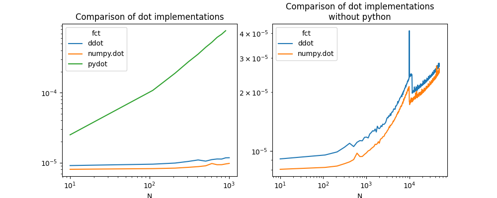
Text(0.5, 1.0, 'Comparison of dot implementations\nwithout python')

The results depends on the machine, its number of cores, the compilation settings of numpy or this module.

plt.show()